8. Technological shift and labour markets

KAT.TAL.322 Advanced Course in Labour Economics

Technological shift and the labour market

This lecture is based on Acemoglu and Autor (2011)

Stylised facts

Labour market of educated workers

Source: Figures 1 and 2 (Acemoglu and Autor 2011)

Labour supply of educated workers grew faster than that of uneducated workers. Contrary to the predictions of standard labour supply and demand theories, the relative wages of educated workers were also growing since the 1980s.

This is typically attributed to technological shift that also increased demand for educated workers.

In this lecture we will study both canonical models of skill-biased technological change and more recent task-based models that allow us to study the question of labour displacement.

Canonical model

Notation

$j\in \{L,MH\}$	Production input
$A_j$	Technology of input $j$
$w_j$	Wages of input $j$
$i$	Production task
$y(i)$	Output of task $i$
${\alpha }_j(i)$	Productivity of input $j$ in task $i$
$j(i)$	Allocation of input $j$ to task $i$
$J\equiv \int j(i)\text{d}i$	Aggregate demand for input $j$
$I_L$	$maxi$ allocated to $L$-type worker
$I_H$	$mini$ allocated to $H$-type worker

Canonical model

Overview

• Two types of labour: high- and low-skill
  Typically, high edu and low edu (can be relaxed)

• Skill-biased technological change (SBTC)
  New technology disproportionately $\uparrow$ high-skill labour productivity

• High- and low-skill are imperfectly substitutable
  Typically, CES production function with elasticity of substitution $\sigma$

• Competitive labour market

Canonical model

Production function

$$Y={[{\left(A_{L}L\right)}^{\frac{\sigma -1}{\sigma }}+{\left(A_{H}H\right)}^{\frac{\sigma -1}{\sigma }}]}^{\frac{\sigma }{\sigma -1}}$$

• $A_L$ and $A_H$ are factor-augmenting technology terms

• $\sigma \in [0,\mathrm{\infty })$ is the elasticity of substitution

  • $\sigma >1$ gross substitutes
  • $\sigma <1$ gross complements
  • $\sigma =0$ perfect complements (Leontieff production)
  • $\sigma \to \mathrm{\infty }$ perfect substitutes
  • $\sigma =1$ Cobb-Douglas production

• We consider production function that only depends on labour input. However, we now differentiate between two types of labour: high-skill $H$ and low-skill $L$.

• Technological changes do not directly replace skills, it simply makes one type of labour more or less productive.

• So, the trends in the labour market over the past decades could be described with $\uparrow A_H$, i.e., high-skill labour becoming more productive.

• It is straightforward to assume that firms would want to shift their production to exploit the greater productivity of the high-skilled labour.

• However, in perfectly competitive labour markets also wages $w_H$ are pushed upwards. Therefore, total impact on equilibrium labour demand $L$ and $H$ depends on the elasticity of substitution $\sigma$.

Canonical model

Rationalisation of CES production function

1. Single output $Y$; $H$ and $L$ are imperfect substitutes
2. Two goods $Y_H=A_{H}H$ and $Y_L=A_{L}L$; CES utility of consumers ${[Y_L^{\frac{\sigma -1}{\sigma }}+Y_H^{\frac{\sigma -1}{\sigma }}]}^{\frac{\sigma }{\sigma -1}}$
3. Combination of the 1. and 2.

Supply of $H$ and $L$ assumed inelastic $\Rightarrow$ study only firm side

There are several rationalisations for the choice of the CES production function.

1. There is single output $Y$ that can be produced by both $H$ and $L$ workers. These workers are imperfect substitutes for each other. For example, all food in a restaurant can be prepared by either a single chef or two waiters.
2. There are in fact two goods $Y_H$ and $Y_L$. Only $H$ workers can produce good $Y_H$ and $L$ workers - $Y_L$ goods. The consumers in the economy perceive the goods $Y_H$ and $Y_L$ as imperfect substitutes for each other. Therefore, we can study the overall employment in this economy using the CES production function without having to model two labour markets.
3. A combination of the two. There are, in fact, two goods $Y_H$ and $Y_L$. Both goods can be produced by both worker types $H$ and $L$. The combined production and labour demand then happens to look like the CES production function.

Also it is important to note that in this model the supply of labour by different types is assumed inelastic. Therefore, it is sufficient to study only the firm behaviour. However, this will only render partial results and full analysis would require us to also consider labour supply and human capital investment decisions.

Canonical model

Equilibrium wages

$$\begin{array}{rl}{w}_L& =A_L^{\frac{\sigma -1}{\sigma }}{[A_L^{\frac{\sigma -1}{\sigma }}+A_H^{\frac{\sigma -1}{\sigma }}{\left(\frac{H}{L}\right)}^{\frac{\sigma -1}{\sigma }}]}^{\frac{1}{\sigma -1}}\\ w_H& =A_H^{\frac{\sigma -1}{\sigma }}{[A_L^{\frac{\sigma -1}{\sigma }}{\left(\frac{H}{L}\right)}^{-\frac{\sigma -1}{\sigma }}+A_H^{\frac{\sigma -1}{\sigma }}]}^{\frac{1}{\sigma -1}}\end{array}$$

Comparative statics:

• $\frac{\partial w_L}{\partial H/L}>0$ low-skill wage rises with $\frac{H}{L}$
• $\frac{\partial w_H}{\partial H/L}<0$ high-skill wage falls with $\frac{H}{L}$
• $\frac{\partial w_i}{\partial A_L}>0$ and $\frac{\partial w_i}{\partial A_H}>0,\mathrm{\forall }i\in \{L,H\}$

You can verify that profit-maximising firm will choose labour demand $L$ and $H$ according to the two equations above. The interpretation is standard: the optimal demand is found at a point where marginal productivity of labour is equal to its marginal cost. Only this time, both marginal productivities and wages are type-specific.

You can also verify the simple comparative statics.

• Wages of the low-type $w_L$ are increasing with the share of high-skilled labour. Since low-skilled labour is shrinking, firms have to compete more with each other to convince the $L$ workers to come work for them.
• Wages of the high-type $w_H$ are decreasing in $\frac{H}{L}$. Since high-skilled labour becomes more abundant, firms do not need to compete as hard for every $H$ worker.
• Both wages are increasing in their respective productivities. If workers become more productive, their wages rise correspondingly in a perfect competition environment.

Canonical model

Skill premium

$$\frac{w_H}{w_L}={\left(\frac{A_H}{A_L}\right)}^{\frac{\sigma -1}{\sigma }}{\left(\frac{H}{L}\right)}^{-\frac{1}{\sigma }}$$

$\mathrm{\Delta }$ relative supply

$$\frac{\partial \ln \frac{w_H}{w_L}}{\partial \ln \frac{H}{L}}=-\frac{1}{\sigma }<0$$

$\mathrm{\Delta }$ technology

$$\frac{\partial \ln \frac{w_H}{w_L}}{\partial \ln \frac{A_H}{A_L}}=\frac{\sigma -1}{\sigma }\lessgtr 0$$

• Gross substitutes: $\sigma >1\Rightarrow \frac{\partial \ln w_H/w_L}{\partial \ln A_H/A_L}>0$
• Gross complements: $\sigma <1\Rightarrow \frac{\partial \ln w_H/w_L}{\partial \ln A_H/A_L}<0$
• Cobb-Douglas: $\sigma =1\Rightarrow \frac{\partial \ln w_H/w_L}{\partial \ln A_H/A_L}=0$

Given the optimality conditions for $w_L$ and $w_H$ we can write down an expression for the skill premium in wages $\frac{w_H}{w_L}$. Using this expression we can analyse the responsiveness of the skill premium with respect to a) changes in relative supply $\frac{H}{L}$ and b) changes in relative productivities $\frac{A_H}{A_L}$.

The skill premium is shrinking with relative supply of high-skilled labour. This is not surprising and also follows from the discussion on the previous slide. However, if you remember the motivating figures at the beginning of the lecture, we saw that relative wages of educated workers rose while their relative supply also increased at the same time. So, it is clear that something else must have been happening at the same time.

The impact of technological innovation on the skill premium depends on the elasticity of substitution between $L$ and $H$.

• If worker types are gross substitutes, then a shift in relative productivity of high-skilled labour $\frac{A_H}{A_L}$ motivates firms to increase their demand for high-skilled labour. So, the skill premium in wages also rises.
• If worker types are gross complements, then the skill premium in wages falls. In this case, $H$ do become more productive, but firms need a specific ratio of inputs from $H$ and $L$ workers to produce output $Y$. Thus, for existing level of $L$ workers, firms require fewer $H$ workers to produce same output $Y$.

The observed patterns in the data are, therefore, consistent with either $H$ and $L$ workers being gross substitutes, or technological shift in the direction $\downarrow \frac{A_H}{A_L}$. The latter is less likely when we think about the nature of technological advancements over the past decades, so the story of gross substitutes sounds more reasonable.

Tinbergen’s race in the data

Katz and Murphy (1992)

The log-equation of skill premium is extremely attractive for empirical analysis

$$\ln \frac{w_{H,t}}{w_{L,t}}=\frac{\sigma -1}{\sigma }\ln \left(\frac{A_{H,t}}{A_{L,t}}\right)-\frac{1}{\sigma }\ln \left(\frac{H_t}{L_t}\right)$$

Assume a log-linear trend in relative productivities

$$\ln \left(\frac{A_{H,t}}{A_{L,t}}\right)={\alpha }_0+{\alpha }_{1}t$$

and plug it into the log skill premium equation:

$$\ln \frac{w_{H,t}}{w_{L,t}}=\frac{\sigma -1}{\sigma }{\alpha }_0+\frac{\sigma -1}{\sigma }{\alpha }_{1}t-\frac{1}{\sigma }\ln \left(\frac{H_t}{L_t}\right)$$

We can use the expression for the skill premium to estimate the parameters in the data. After taking logs on both sides and assuming log-linear trend in innovation, we can express log skill premium as a function of time trend $t$ and relative labour supply $\frac{H}{L}$.

$$\ln \frac{w_{H,t}}{w_{L,t}}={\beta }_0+{\beta }_{1}t+{\beta }_2\ln \frac{H_t}{L_t}+u_t$$

We can use time-series data from the labour markets to estimate the regression and back out $\hat{\sigma }$ from $\widehat{{\beta }_2}$.

Tinbergen’s race in the data

Katz and Murphy (1992)

Estimated the skill premium equation using the US data in 1963-87 $$\ln {\omega }_t=\text{cons}+\underset{(0.005)}{0.027}\times t-\underset{(0.128)}{0.612}\times \ln \left(\frac{H_t}{L_t}\right)$$

Implies elasticity of substitution $\sigma \approx \frac{1}{0.612}=$ 1.63

Agrees with other estimates that place $\sigma$ between 1.4 and 2 (Acemoglu and Autor 2011)

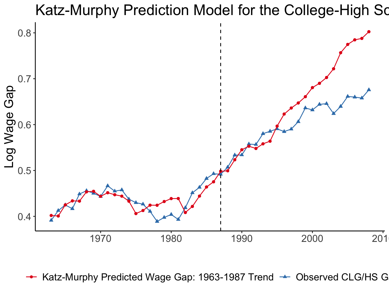
Tinbergen’s race in the data

Source: Figure 19 (Acemoglu and Autor 2011)

Very close fit up to mid-1990s, diverge later

Fit up to 2008 implies $\sigma \approx$ 2.95

Accounting for divergence:

• non-linear time trend in $\ln \frac{A_H}{A_L}$
  brings $\sigma$ back to 1.8, but implies $\frac{A_H}{A_L}$ slowed down

• differentiate labour by age/experience as well

Using the estimated regression, we can also plot the predicted and observed skill premium over time. The red curve corresponds to predicted skill premium from the estimation based on 1963-1987. The vertical red line marks the end of the estimation period. So, we can see that observed and predicted skill gap are very close to each both in- and out-of sample until mid-1990s. But the series start diverging from early 2000s.

If the entire period until 2008 is used for estimation, then the implied $\sigma \approx$ 2.95, which is substantially higher than most of the estimates in the literature.

The divergence can be explained in the context of the canonical model in two ways.

1. Technological progress is non-linear and started to decelerate in 2000s. While the idea of non-linear technological progress can be sensible, it is hard to believe that it slowed down in the last three decades! So, it is not a reasonable explanation for the flattening of the skill premium.
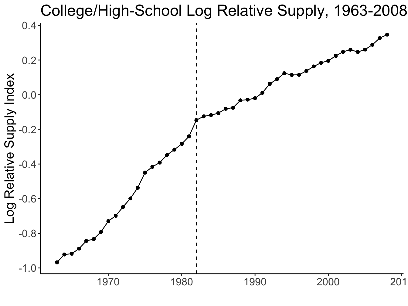
2. Relative supply of skilled labour has changed. In the model we assumed the supply doesn’t change. Obivously, in real life, it also responds to market incentives and policy changes. The aggregate relative supply of college-educated workers increased over time, but it might have happened heterogeneously in different experience groups. For example, there were fewer men getting college degree after the end of Vietnam war, which shows up as lower relative supply of experienced college-educated workers twenty years later. Therefore, Acemoglu and Autor (2011) estimate the skill premium regression with aggregate and experience-group-specific labour supply. This helps improve the fit for the entire period.

Canonical model

Summary

1. Simple link between wage structure and technological change
2. Attractive explanation for college/no college wage inequality¹
3. Average wages $\uparrow$ (follows from $\partial w_i/\partial A_H$ and $\partial w_i/\partial A_L$)

However, the model cannot explain other trends observed in the data:

1. Falling $w_L$
2. Earnings polarization
3. Job polarization

Also silent about endogeneous adoption or labour-replacing technology.

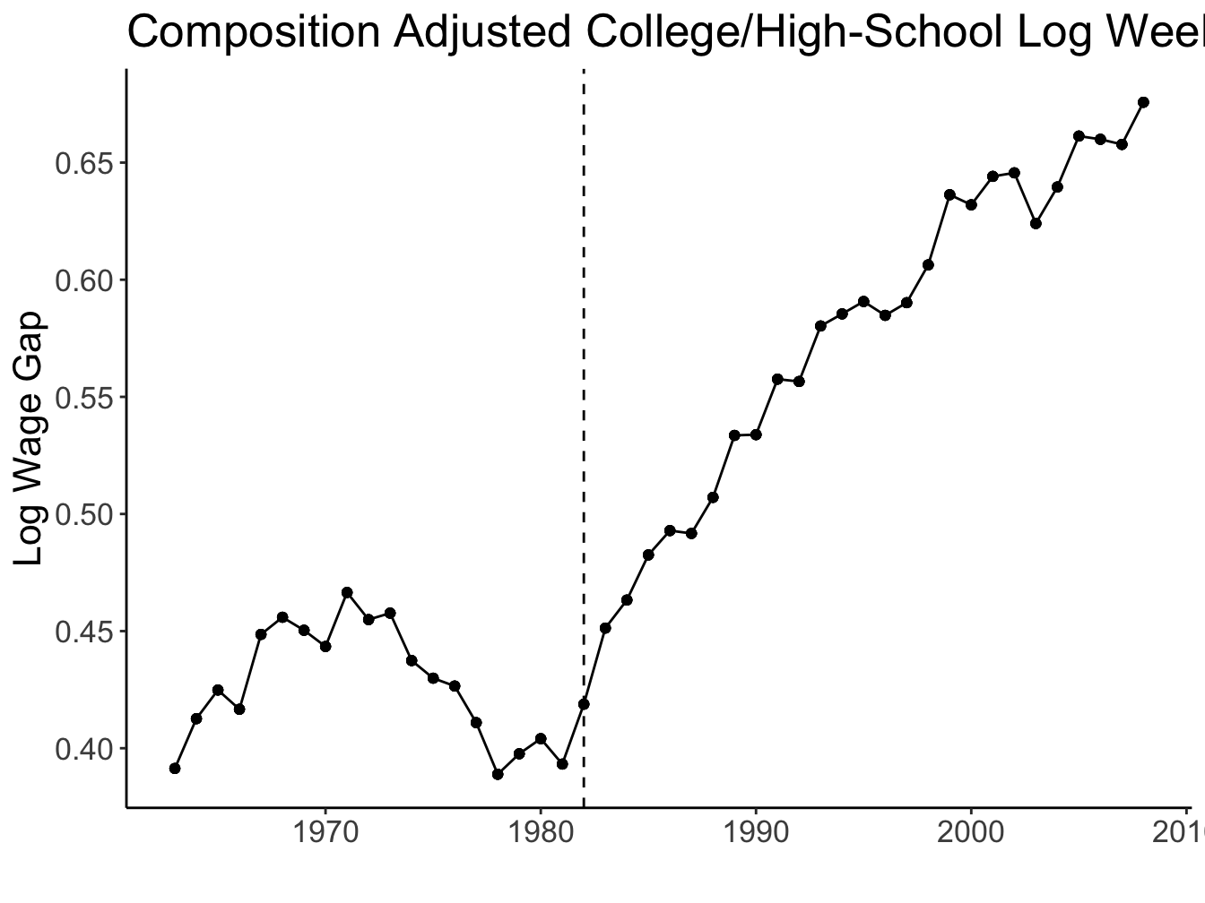
Unexplained trend: falling real wages

Source: Figure 1 (Autor 2019)

The skill premium in wage can increase because either

• wage level of high-skill workers rise, or
• wage level of low-skill workers fall, or
• both.

The figure above shows that infact the rising skill premia is the combination of the two: the wage level of college-educated workers rose, while that of high-school dropouts fell over time.

If we go back to the comparative statics of wage levels, we can see that the only way $w_L$ falls in the canonical model is if

• $\downarrow \frac{H}{L}$ (which is refuted by the motivating picture at the beginning of the lecture), or
• $\downarrow A_L$ or $\downarrow A_H$ (which implies technological regress in either low- or high-skilled tasks).

Both of these are hard to believe in. We have explicitly shown that $\frac{H}{L}$ has been steadily rising since mid-XX century. And even though we are willing to assume that technological progress happened more rapidly in high-skilled tasks, it is unreasonable to assume that productivity of low-skilled labour was declining. If anything, productivity of low-skilled labour has also increased thanks to the machines that can do very routine tasks faster, easier, maybe more efficiently.

Therefore, we must conclude that the canonical model does not fit all the data patterns and that we need a different type of model.

Unexplained trend: earnings polarization

Source: Figure 8 (Acemoglu and Autor 2011)

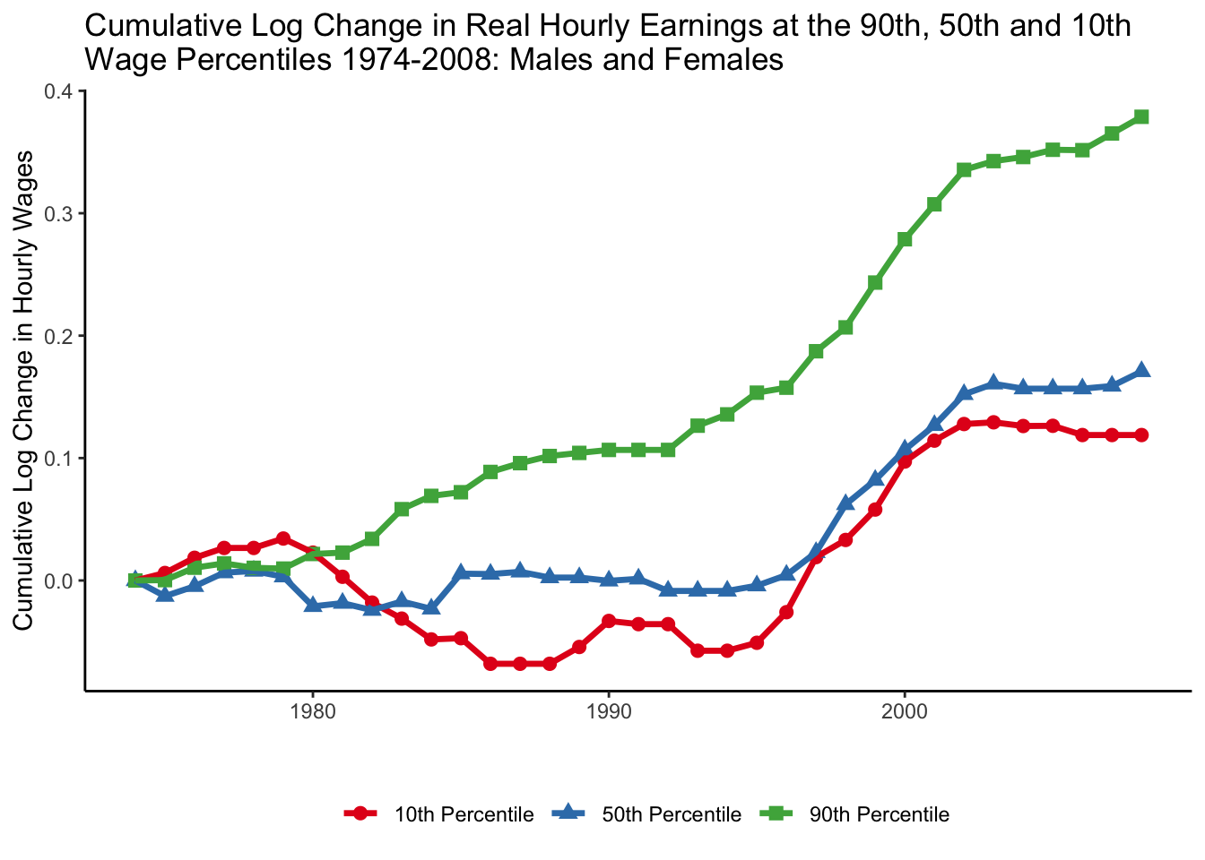
The canonical model can explain between group inequality, like college vs non-college workers ($\frac{w_H}{w_L}$). However, it cannot say anything about inequality within groups.

The figure above shows the evolution of log hourly earnings at the bottom (10th percentile), middle (50th percentile) and top (90th percentile) of the earnings distribution. We can see that earnings at the top were growing much faster than the rest of the distribution. Earnings in the middle remained roughly flat until the 2000s and earnings at the bottom had brief period of reduction in the 1980s. These trends suggest that also inequality within groups might have evolved in different ways.

Unexplained trend: job polarization

Source: Figure 10 (Acemoglu and Autor 2011)

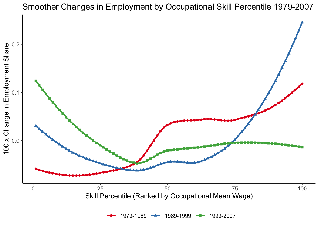
The canonical skill-biased technological change (SBTC) model also cannot explain the phenomenon of job polarization: wages and employments in low- or high-skilled jobs grow faster than in mid-skilled jobs. We need a model that explicitly incorporates tasks to be able to study these kinds of questions.

Task-based model

Task-based model

Overview

Task is a unit of work activity that produces output

Skill is a worker’s endowment of capabilities for performing tasks

Key features:

1. Tasks can be performed by various inputs (skills, machines)
2. Comparative advantage over tasks among workers
3. Multiple skill groups
4. Consistent with canonical model predictions

The crucial feature of task-based model is the separation between worker skill and job tasks. Here, tasks are specific units of work activities that need to be done to produce the output. For example, buying ingrediants, making a dough and baking a bun could be two tasks that describe the job of a baker. Worker’s skills allow her to do these tasks with varying level of competence. For example, worker A who is particularly skilled at econometrics might not be that good in baking a bun. If you think about it then you may conclude that worker skills are basically measures of their relative advantages. That is exactly how the task-based model is presented in Acemoglu and Autor (2011).

• This framework allows us to specify the production function such that a task can be produced by either a worker with some skills or machines (so, we could study labour-replacing technology).
• Since workers’ skills determine their relative advantage in doing any given task, we can also study endogenous allocation of workers to jobs.
• We can study job polarisation with this model (need to have at least 3 skill groups for that).
• Finally, this model is consistent with the canonical SBTC model. If we equate job tasks to worker skills, we will get the canonical SBTC model.

Task-based model

Production function

Unique final good $Y$ produced by continuum of tasks $i\in [0,1]$

$$Y=\exp [{\int }_0^1\ln y(i)\text{d}i]$$

Three types of labour: $H$, $M$ and $L$ supplied inelastically.

$$y(i)=A_L{\alpha }_L(i)l(i)+A_M{\alpha }_M(i)m(i)+A_H{\alpha }_H(i)h(i)+A_K{\alpha }_K(i)k(i)$$

• $A_L,A_M,A_H,A_K$ are factor-augmenting technologies

• ${\alpha }_L(i),{\alpha }_M(i),{\alpha }_H(i),{\alpha }_K(i)$ are task productivity schedules

• $l(i),m(i),h(i),k(i)$ are production inputs allocated to task $i$

Fir simplicity, assume ${\alpha }_K(i)=0,\mathrm{\forall }i\in [0,1]$. See Acemoglu and Restrepo (2018) for a more complete analysis of the model.

We first begin by describing the production function. Now, an output $Y$ is not produced by just a unit of labour or capital, rather by certain tasks $i$. For simplicity, let’s assume that there is a continuum of tasks that can be ranked in a range $[0,1]$. Each task produces “intermediate” output $y(i)$. For simplicity, we also assume Cobb-Douglas technology. If tasks were discrete we could have written $Y=y(0)\cdot y(1)\cdot \dots \cdot y(n)$. The above expression is an equivalent of this idea with continuous tasks.

We assume there are three types of labour: high-skilled $H$, medium-skilled $M$ and low-skilled $L$. Any task $i$ can be performed by all three types of workers, albeit with different productivities. In addition, we allow same task to be produced by machines. For now, let’s keep assuming inelastic supply of labour of each type. Check out Section 4.6 in Acemoglu and Autor (2011) for the discussion of the model with endogenous supply of skills.

The $\{A_L,A_M,A_H,A_K\}$ capture the factor-augmenting technology, while $\{{\alpha }_L(i),{\alpha }_M(i),{\alpha }_H(i),{\alpha }_K(i)\}$ capture comparative advantages of the production inputs in performing task $i$. So, an increase in ${\alpha }_L(i)$ would mean that $L$-type worker became more efficient at performing a given task $i$; whereas an increase in $A_L$ means that $L$-type worker became more efficient at performing all tasks $i\in [0,1]$.

Finally, the terms $\{l(i),m(i),h(i),k(i)\}$ capture the allocation of each input factor to a given task $i$. This allocation is firm’s decision that it makes when maximising

For simpler illustration of the model, we assume that ${\alpha }_K(i)=0,\mathrm{\forall }i$. But we will consider later a case where it is non-zero and is more efficient than any labour type at certain range of tasks.

Task-based model

Comparative advantage assumption

${\alpha }_L(i)/{\alpha }_M(i)$ and ${\alpha }_M(i)/{\alpha }_H(i)$ are continuously differentiable and strictly decreasing.

Market clearing conditions

$${\int }_0^{1}l(i)\text{d}i\le L{\int }_0^{1}m(i)\text{d}i\le M{\int }_0^{1}h(i)\text{d}i\le H$$

Continuously differentiable $\frac{{\alpha }_L(i)}{{\alpha }_M(i)}$ and $\frac{{\alpha }_M(i)}{{\alpha }_H(i)}$ is a regularity assumption that allows us to easily study the comparative statics in this model.

The relative productivities are decreasing in $i$ which means that higher-skilled labour has comparative advantage in more difficult tasks. We do not make an assumption on productivity schedules themselves. For example, it can be that all three types of workers are more productive at higher-level tasks ${\alpha }_j^{\prime }(i)>0,\mathrm{\forall }j\in \{L,M,H\}$. But the important thing is that productivity of $M$-type worker rises faster than $L$-type worker, and that of $H$-type worker - faster than $M$-type worker. Therefore, ratios $\frac{{\alpha }_L(i)}{{\alpha }_M(i)}$ and $\frac{{\alpha }_M(i)}{{\alpha }_H(i)}$ are decreasing in $i$.

Task-based model

Equilibrium without machines

Lemma 1

Given comparative advantage assumption, there exist $I_L$ and $I_H$ such that

Note that boundaries $I_L$ and $I_H$ are endogenous

This gives rise to the substitution of skills across tasks

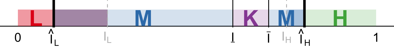
Given the way we described comparative advantages, we can make a conjecture that in equilibrium there are threshold tasks $I_L$ and $I_H$ such that firm uses

• only $L$-type workers for tasks $i\le I_L$,
• only $M$-type workers for tasks $I_L<i\le I_H$, and
• only $H$-type workers for tasks $i>I_H$.

Since it is the firm that chooses these treshholds, we can study the substitution of skills across tasks in response to changes in the envirionment. For example, if a relative supply of $H$ skills increases, their wages $w_H$ should fall. That means that firms could allocate $H$-type workers to larger set of tasks ($\downarrow I_H$) since we assume that $H$-type workers are more productive than $M$-type workers. Alternatively, we can also study the implications of technological progress that raises $A_H$ or ${\alpha }_H(\cdot )$.

Task-based model

Law of one wage

Output price is normalised to 1 $\Rightarrow \exp [{\int }_0^1\ln p(i)\text{d}i]=1$

All tasks employing a given skill pay corresponding wage

$$\begin{array}{rl}{w}_L& =p(i)A_L{\alpha }_L(i),\mathrm{\forall }i\in [0,I_L]\\ w_M& =p(i)A_M{\alpha }_M(i),\mathrm{\forall }i\in (I_L,I_H]\\ w_H& =p(i)A_H{\alpha }_H(i),\mathrm{\forall }i\in (I_H,1]\end{array}$$

See Appendix: derivation of wage equations

Task-based model

Skill allocations

Given the law of one wage, we can show that

$$\begin{array}{rlrl}l(i)& =l\left(i^{\prime }\right)& \Rightarrow & l(i)=\frac{L}{I_L}\mathrm{\forall }i\in [0,I_L]\\ m(i)& =m\left(i^{\prime }\right)& \Rightarrow & m(i)=\frac{M}{I_H-I_L}\mathrm{\forall }i\in (I_L,I_H]\\ h(i)& =h\left(i^{\prime }\right)& \Rightarrow & h(i)=\frac{H}{1-I_H}\mathrm{\forall }i\in (I_H,1]\end{array}$$

See Appendix: derivation of skill allocations

Task-based model

Endogenous thresholds: no arbitrage

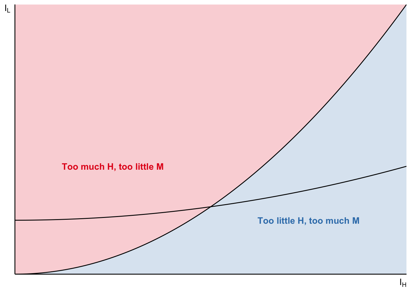
Threshold task $I_H$: equally profitable to produce with either $H$ or $M$ skills

$$\frac{A_M{\alpha }_M(I_H)M}{I_H-I_L}=\frac{A_H{\alpha }_H(I_H)H}{1-I_H}$$

Similarly, for $I_L$:

$$\frac{A_L{\alpha }_L(I_L)L}{I_L}=\frac{A_M{\alpha }_M(I_L)M}{I_H-I_L}$$

Using same logic as in Appendix: derivation of skill allocations, we know that

$$p(i)y(i)=p\left(i^{\prime }\right)y(\left(i^{\prime }\right),\mathrm{\forall }i\in [0,I_L],i^{\prime }\in (I_L,I_H]$$

This equality is useful also to pin down the values of thresholds

$$\begin{array}{rl}p(I_L)A_L{\alpha }_L(I_L)\frac{L}{I_L}& =p(I_L)A_M{\alpha }_M(I_L)\frac{M}{I_H-I_L}\\ p(I_H)A_H{\alpha }_H(I_H)\frac{H}{1-I_H}& =p(I_H)A_M{\alpha }_M(I_H)\frac{M}{I_H-I_L}\end{array}$$

Hence, the equations in the above slide.

Task-based model

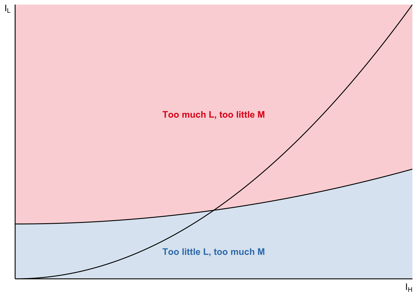
Endogenous thresholds: no arbitrage

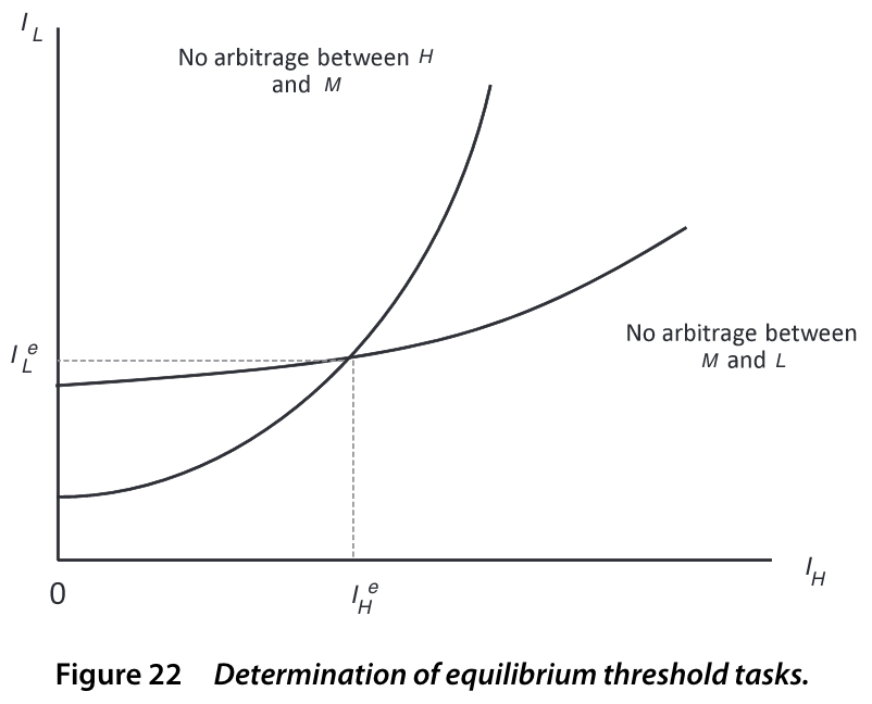
The equilibrium at the intersection because that’s when firm has no incentive to use $M$ for either of $L$ or $H$ tasks. Consider another point along H-M curve: firm is still indifferent between $H$ and $M$ for $I_H$ task. But there will be arbitrage where $M$ could be more profitable for $I_L$ task (or $L$).

Task-based model

Comparative statics: wage elasticities

$$\begin{array}{ccc}\frac{\text{d}\ln w_H/w_L}{\text{d}\ln A_H}>0& \frac{\text{d}\ln w_M/w_L}{\text{d}\ln A_H}<0& \frac{\text{d}\ln w_H/w_M}{\text{d}\ln A_H}>0\\ \frac{\text{d}\ln w_H/w_L}{\text{d}\ln A_M}⪋0& \frac{\text{d}\ln w_M/w_L}{\text{d}\ln A_M}>0& \frac{\text{d}\ln w_H/w_M}{\text{d}\ln A_M}<0\\ \frac{\text{d}\ln w_H/w_L}{\text{d}\ln A_L}<0& \frac{\text{d}\ln w_M/w_L}{\text{d}\ln A_L}<0& \frac{\text{d}\ln w_H/w_M}{\text{d}\ln A_L}>0\end{array}$$

Task-based model

Comparative statics: $\uparrow A_H$

Source: Figure 25 (Acemoglu and Autor 2011)

An increase in $A_H$ means that $H$-type workers become more productive at every task.

• So, the firm wants to let $H$-type workers handle more tasks $\Rightarrow \downarrow I_H$.
• This means that $M$-type workers are now in excess, which means their wages are pushed down $\Rightarrow \downarrow \frac{w_M}{w_L}$.
• Since $M$-type workers are more productive than $L$-type workers and they become cheaper, firms also find it useful can now also perform some of the tasks previously done by $L$-type workers in a profitable way $\Rightarrow \downarrow I_L$.
• This also means that $L$-type workers are over-supplied now, which pushes their wages down too. Therefore, the set of tasks for which $L$-type workers are more profitable for the firm does not shrink quite as much.
• Overall, the wages of $M$-type workers have to go down considerably more than wages of $L$-type workers.

Notice that the sign of the comparative statics with respect to change in $A_M$ is not entirely determined by the model assumptions. When $\uparrow A_M$, $M$-type workers are more productive at every task. So, it will simultaneously push $\uparrow I_H$ and $\downarrow I_L$. This means that both $H$-type and $L$-type workers are over-supplied and their wages go down. However, depending on the functional form of $\frac{{\alpha }_L(i)}{{\alpha }_M(i)}$ and $\frac{{\alpha }_M(i)}{{\alpha }_H(i)}$, the threshold tasks might shift by different amounts. So, if $|\mathrm{\Delta }{I}_H|>|\mathrm{\Delta }{I}_L|$, the set of tasks allocated to $H$-type workers shrinks a lot more than those allocated to $L$-type workers. Therefore, $\downarrow \downarrow w_H$ and $\downarrow w_L$. However, if $M$-type workers displace $L$-type workers more, then $\downarrow w_H$ and $\downarrow \downarrow w_L$.

Unlike canonical model, changes in $A$ terms can reduce relative wages! More than that, it is also possible to show they reduce absolute levels of wages too (Wage effects in subsection 4.4)

Curiosity time

Can you derive comparative statics with respect to labour supply levels $L,M$ and $H$? Can you also come up with intuition?

Task-based model

Task replacing technologies

Start from initial equilibrium without machines

Assume in $[\underset{―}{I},\overline{I}]\subset [I_L,I_H]$ machines outperform $M$. Otherwise, ${\alpha }_K(i)=0$.

How does it change the equilibrium?

Now, let’s consider what happens to the equilibrium when technological innovation is not factor-augmenting, but labour-replacing. In this example, we consider a case when machines can now out-perform $M$-type workers in some of their tasks. The current case is consistent with automation of routine tasks in Autor, Levy, and Murnane (2003).

Curiosity time

Machines can replace tasks anywhere on $[0,1]$. Try to analyse alternative cases where machines replace $H$-type workers or $L$-type workers.

Let’s say the tasks that can be replaced by machines are in the interval $[\underset{―}{I},\overline{I}]\subset [I_L,I_H]$. How does equilibrium change now?

Task-based model

Task replacing technologies

Assume comparative advantage of $H$ over $M$ stronger than $M$ over $L$

1. $w_H/w_M$ increases
2. $w_M/w_L$ decreases
3. $w_H/w_L\uparrow (\downarrow )$ if $|{\beta }_L^{\prime }(I_L)I_L|\stackrel{<}{>}|{\beta }_H^{\prime }(I_H)(1-I_H)|$

1. Machines replace $M\Rightarrow$ demand for $M$-type worker $\downarrow \Rightarrow w_M\downarrow$
2. Now, the excess supply of $M$-type workers is redeployed to other tasks: they take over some tasks that were previously done by $L$-type workers and also some tasks done by $H$-type workers. Let old thresholds be denoted $I_L$ and $I_H$, and new ones - ${\hat{I}}_L$ and ${\hat{I}}_H$. Then, we can show that ${\hat{I}}_H-{\hat{I}}_L\ge I_H-I_L$.
3. Here, we assume that comparative advantage of $M$-type workers are more readily substitutable with $L$-type workers than $H$-type workers. Therefore, the firms would prefer to re-deploy the $M$-type workers to tasks done by $L$-type workers to a larger extent than those done by $H$-type workers. This means that $|{\hat{I}}_H-I_H|\le |{\hat{I}}_L-I_L|$.

What does it mean for wages?

1. We know that wages of $M$-type workers, $w_M$, fall. Actually, we can show that relative wages with respect to both $w_L$ and $w_H$ fall. So, wages of the displaced workers fall the most!
2. We have argued above that $M$-type workers, in turn, displace $L$-type workers more than $H$-type workers. This means that over-supply of $L$-type workers is more severe than that of $H$-type workers. Therefore, relative wages $\uparrow \frac{w_H}{w_L}$.

Thus, we can see how skill-replacing technological advancement can generate both

• fall in real wages, and
• disproportionate fall in $w_M$ compared to smaller changes in $w_L$ and $w_H$.

Task-based model

Endogenous supply of skills

Each worker $j$ is endowed with some amount of each skill $l^j,m^j,h^j$

Workers allocate time to each skill given

$$\begin{array}{rl}& t_l^j+t_m^j+t_h^j\le 1\\ & w_L{t}_l^j{l}^j+w_M{t}_m^j{m}^j+w_H{t}_h^j{h}^j\end{array}$$

Comparative advantage: $\frac{h^j}{m^j}$ and $\frac{m^j}{l^j}$ are decreasing in $j$

Then, there exist $J^{\star }\left(\frac{w_H}{w_M}\right)$ and $J^{\star \star }\left(\frac{w_M}{w_L}\right)$

So far, we have assumed inelastic labour supply, which gave us valuable insights. But to consider full implications of the technological changes, we need to take into account changes in the supply of skills. If the incentives changed such that $M$ skills are not as attractive anymore, workers can re-train and direct their human capital towards $L$ or $H$ skills.

Consider some worker $j$. From birth she is endowed with a vector of skills $(l^j,m^j,h^j)$. At every point in time she is endowed with one unit of time, that she needs to split between supplying the three types of skills on the labour market. Maybe you can imagine that she can choose to work three jobs: one that uses $L$ skills, another - $M$ skills, and third - $H$ skills. She can for example, work 20% of time in first job, 20% - in second and 60% - in third. Her time allocations are captured by vector $(t_l^j,t_m^j,t_h^j)$.

Let’ assume, again for simplicity, that she has linear risk-neutral utility with no disutility of labour. Therefore, her utility is equivalent to her earnings

$$w_L{t}_l^j{l}^j+w_M{t}_m^j{m}^j+w_H{t}_h^j{h}^j$$

The labour supply, therefore, is

$$L=\int l^j\text{d}jM=\int m^j\text{d}jH=\int h^j\text{d}j$$

We also assume that workers have their comparative advantages in the three skill types. In particular, we impose an order on $j$ such that $\frac{h^j}{m^j}$ and $\frac{m^j}{l^j}$ are decreasing in $j$. This assumption, basically, says that lower-indexed workers have comparative advantage in higher-level skills.

Similar to the problem on the firm side, we can make a conjecture that an equilibrium in this model is described by two threshold values $J^{\star }$ and $J^{\star \star }$ such that

$$\{\begin{array}{ll}{t}_h^j=1,& \mathrm{\forall }j\le J^{\star }\\ t_m^j=1,& \mathrm{\forall }{J}^{\star }<j\le J^{\star \star }\\ t_l^j=1,& \mathrm{\forall }j>J^{\star \star }\end{array}$$

Let’s try to reason now, how would endogenous supply react to labour-replacing technology from the previous slide.

It is also reasonable to assume, as we did on the previous slide, that the margin between $M$ and $L$ skills is more responsive than margin between $M$ and $H$ skills. Basically, if $M$ skills become less attractive, the workers who previously supplied $M$ skills will now start supplying more of $L$ skills rather than $H$ skills.

In this case, the total effect on employment of $M$-type workers is even more negative. We have seen already that demand for $M$-type workers falls following the technology that takes over some of their old tasks. Because of this, and negative effect on wages $w_M$, workers find $M$ skills less appealing. So, the displaced $M$-type workers now decide to supply $L$ skills instead. So, also labour supply of $M$-type workers goes down. The overall effect on wages depends on whether demand fell harder than supply.

Now, the over-supply of $L$-type workers is even stronger. Not only the existing $L$-type workers had fewer tasks to do, so had to agree for lower wages to keep jobs, now there are even more of $L$-type workers. This depresses their wages even further $\downarrow w_L$.

So, with endogenous labour supply, we can come up with a reasonable set of assumptions for model parameters that generate disproportionate growth of employment and wages at the extremes of distribution. Employment and wages in the middle fall substantially, while employment and wages at the bottom and top increase (or don’t fall).

Of course, the full set of comparative statics is more difficult in this case and there are fewer clear predictions that the model can make. But it is still easy to see the potential of these type of models in explaining a wide set of patterns in the data. For more detailed discussion and derivations, check Section 4.6 in Acemoglu and Autor (2011)!

Task-based model

Illustration in the data

Suppose $\uparrow A_H\Rightarrow \uparrow \frac{w_H}{w_M},\downarrow \frac{w_M}{w_L}$.

Use occupational specialization at some $t=0$ as comparative advantage.

• ${\gamma }_{sejk}^i$ share of 1959 population employed in $i$ occupations, $\mathrm{\forall }i\in \{H,M,L\}$

$$\mathrm{\Delta }{w}_{sejk\tau }=\sum _t[{\beta }_t^H{\gamma }_{sejk}^H+{\beta }_t^L{\gamma }_{sejk}^L]1\{\tau =t\}+{\delta }_{\tau }+{\varphi }_e+{\lambda }_j+{\pi }_k+e_{sejk\tau }$$

Descriptive regression informed by the model!

It is clear so far that a task and skills allocations are endogenously determined. So, if we try to estimate the relationship between jobs and wages in the observational data, we will not be able to uncover the model parameters. However, it may still prove to be a useful descriptive analysis.

Recall our comparative statics about $\uparrow A_H$. We have argued that relative wages $\frac{w_H}{w_M}$ increase since $H$-type workers are generally more productive now, and that $\frac{w_M}{w_L}$ decrease since over-supply of $M$-type workers is more severe than that of $L$-type workers.

To track these kinds of changes, we can study the evolution of wages in three different sill groups. Suppose we have data with wages $w$ of workers along with information about their gender $s$, education $e$, age-group $j$, region $k$ observed in period $\tau$. Let $\mathrm{\Delta }{w}_{sejk\tau }\equiv w_{sejk\tau }-w_{sejk0}$ denote the change in wage level of the respective population group at period $\tau$ relative to some initial period $0$.

We now need to define variables that capture the comparative advantages of workers in either $L$, $M$, or $H$ skills. This is typically not observed. However, Acemoglu and Autor (2011) suggest we can use specialisation of a certain population group in $L$-, $M$- or $H$-type occupations at the initial period 0 as a proxy for the comparative advantage. We nowadays have some information about tasks performed in all jobs, which we can use to classify the occupations into those types. So, if, say, young college-educated women were more likely to work in high-skilled occupations, we assume they have comparative advantage in those skills. Let ${\gamma }_{sejk}^i,\mathrm{\forall }i\in \{L,M,H\}$ capture share of population group $sejk$ in occupation type $i$ at the initial period 0. Notice that fixing comparative advantages at time 0 may help limit the endogeneity issue between labour demand for skills and labour supply of skills.

Thus, we can regress the $\mathrm{\Delta }{w}_{sejk\tau }$ on ${\gamma }_{sejk}^L$ and ${\gamma }_{sejk}^H$. Given the model predictions, we would expect ${\beta }_t^L$ and ${\beta }_t^H$ to be positive. That is, wages of both $L$-type workers and $H$-type workers rose relative to wages of $M$-type workers.

Task-based model

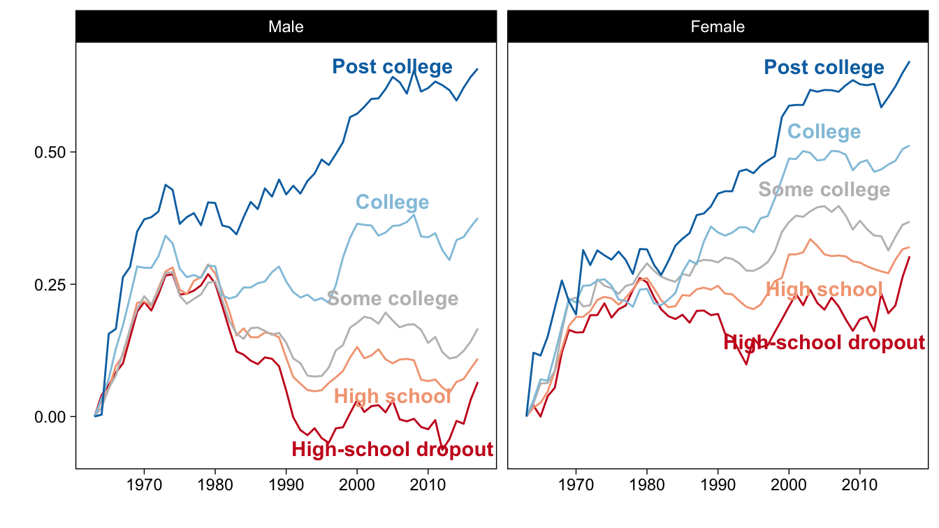
Illustration in the data

Source: Table 10 (Acemoglu and Autor 2011)

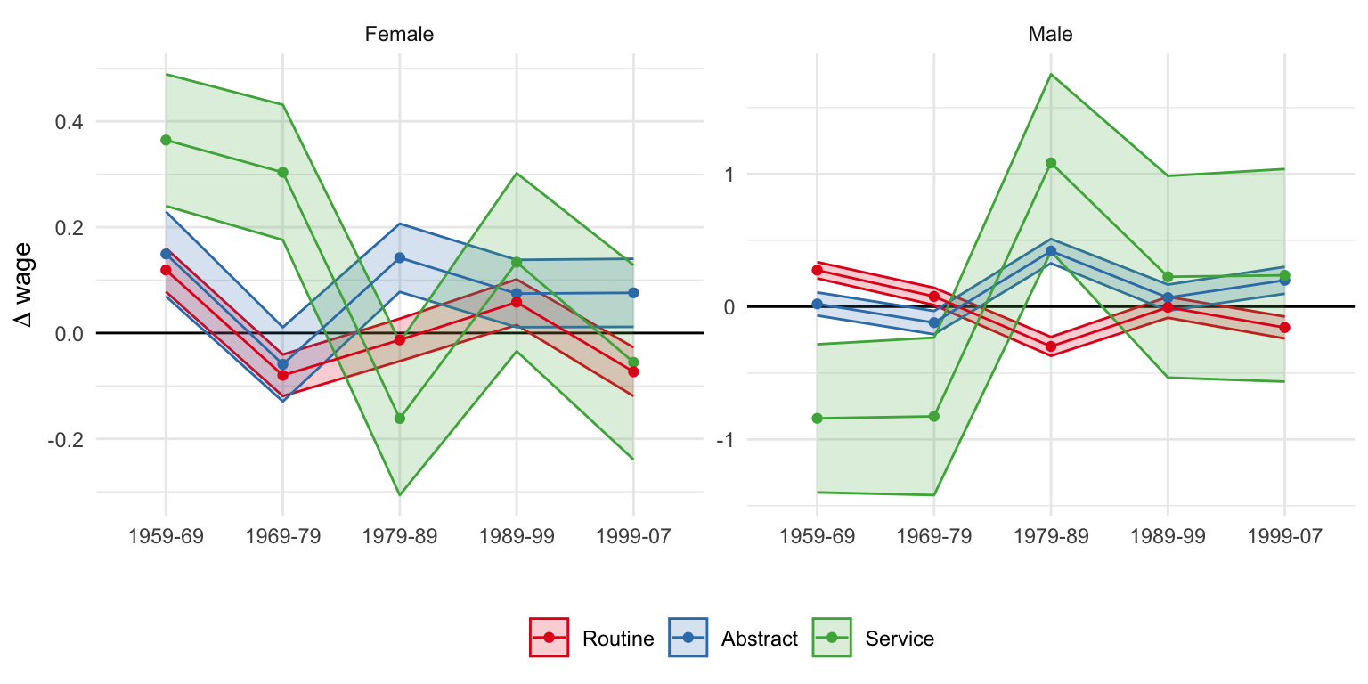
The figure above plots the regression results from Table 10 in Acemoglu and Autor (2011).

One common way of categorizing occupation is if they use abstract ($H$), routine ($M$) or manual ($L$) skills. We can see that both for men and women, wages in abstract occupations rose over time, while wages of those specialised in routine occupations fell. The results for wages of workers specialised in manual occupations has less clear pattern: it rises strongly in the short-term for women, falls for me; eventually, doesn’t really change over four decades.

These results do provide some suggestive evidence that the task-based model can explain patterns seen in the data. However, this is highly descriptive: there is no exogenous variation of skill allocations of either workers or firms; the specialisations at $\tau =0$ may not capture the comparative advantages well and these too can evolve over time.

Task-based model

Summary

1. A rich model that can accommodate numerous scenarios
   1. Outsourcing tasks to lower-cost countries
   2. Endogenous technological change
   3. Creation of new tasks
2. Useful tool to study effect on inequality and job polarization

Empirical results

Acemoglu and Restrepo (2022)

Environment

Multi-sector model with imperfect substitution between inputs

$${\text{Task displacement}}_g^{\text{direct}}=\sum _{i\in \mathcal{I}}{\omega }_g^i\frac{{\omega }_{gi}^R}{{\omega }_i^R}(-d\ln s_i^{L,\text{auto}})$$

• ${\omega }_g^i$ - share of wages earned by worker group $g$ in industry $i$
  (exposure to industry $i$)at $t=0$

• $\frac{{\omega }_{gi}^R}{{\omega }_i^R}$ - specialization of group $g$ in routine tasks $R$ within industry $i$ at $t=0$

• $-d\ln s_i^{L,\text{auto}}$ - % decline in industry $i$’s labour share due to automation

  1. attribute 100% of the decline to automation

  2. predict given industry adoption of automation technology

Source: Figure 4 (Acemoglu and Restrepo 2022)

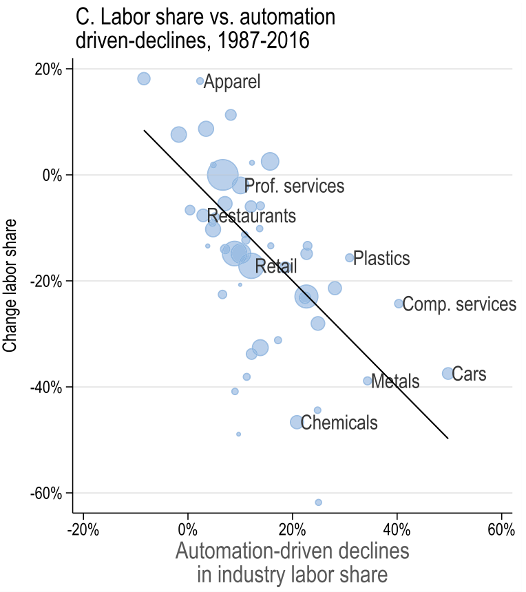
This is a more recent empirical study of the effect of task displacement technologies on employment and wages. The authors focus on period between 1980 and 2016 and construct task displacement index using initial industry specialisations and overall decline in labour share attributed to automation.

• The specialisations are constructed from industry-level. Some industries were hit harder by automation (for example, robotisation in manufacturing sectors) than others. So, authors use exposure of certain population group $g$ to industries as weights.
• The automation is thought to mainly replace routine tasks. Therefore, worker groups that specialise in routine tasks are the one to be affected the most. Recall our discussion earlier in the lecture.
• Finally, we need a measure of how strongly automation affected a given industry over some period. The authors use decline in labour share and either attribute all of it to automation, or only part of it proportional to industry adoption of robotics.

Acemoglu and Restrepo (2022)

Task displacement

Source: Figure 5

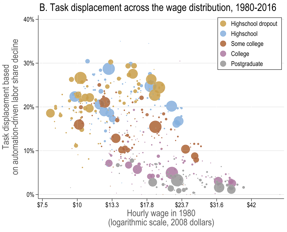
The above figure plots the task displacement index against initial wages by education group of workers. So, it is easy to see that lower-earning workers had higher exposure to task displacing technologies. But notice an inverse U-shape: it is mostly workers towards the middle of wage distribution that experienced largest displacement. We also see correlation with skill measures of workers: higher-education workers have lower task displacement indices even at similar wage levels. This is consistent with our theoretical discussion in Task replacing technologies.

Acemoglu and Restrepo (2022)

Task displacement and changes in real wages

Source: Figure 6 (Acemoglu and Restrepo 2022)

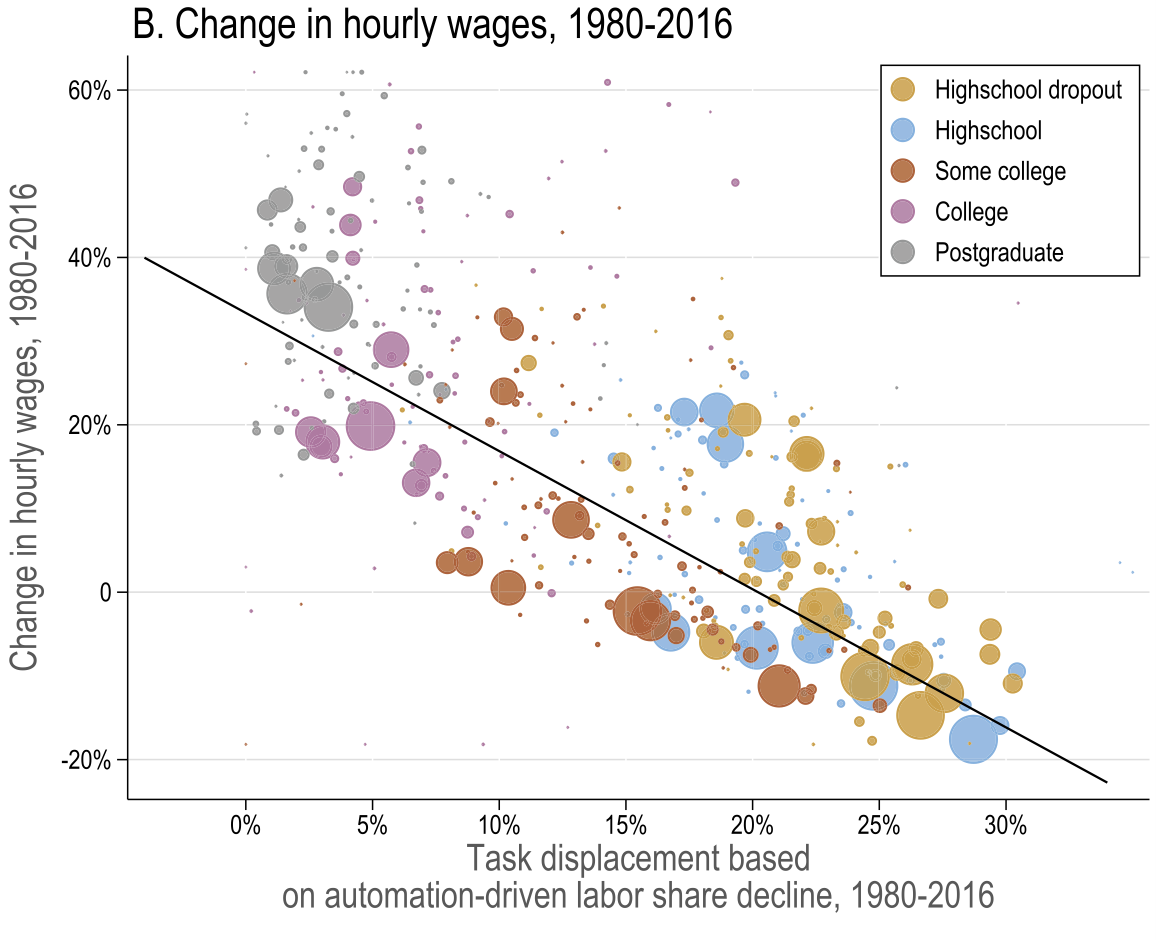
They verify these observations in a series of reduced form regressions. In particular,

• 50-70% of changes in wage structure are linked to task displacement and to a much smaller extent to offshoring

• they conclude that SBTC without task displacement explains less of variation in the data

• they ruled out alternative channels like

  • other non-automation capital

  • increase in capital use intensity

  • markups

  • industry concentration

  • unionization

  • and import competition

However, the reduced form estimates ignore general equilibrium. That is, it assumes

• there is no endogenous adjustment of task thresholds at other margins (ripple effects)

• no change in industry composition

• doesn’t take into account productivity gains

Acemoglu and Restrepo (2022)

General equilibrium results

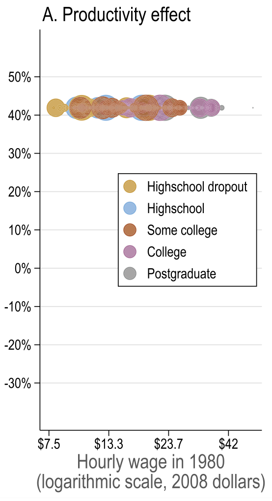
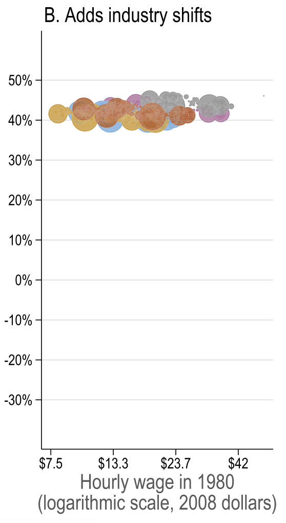
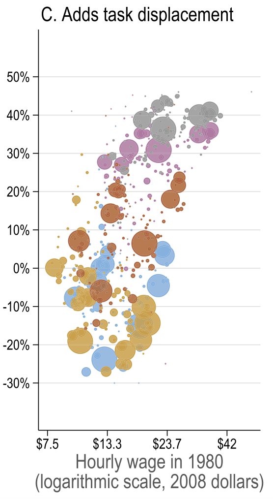
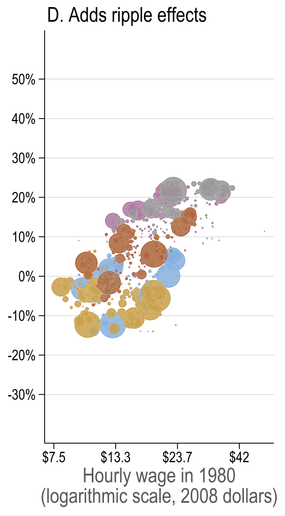
Source: Figure 7 (Acemoglu and Restrepo 2022)

1. Common productivity effect
   It’s when productivity improvement shifts supply of goods upwards meaning that output of firms goes up and as a result firm’s labour demand goes up as well for all labour categories.
2. Changes in industry composition induced by automation
   Automation induces shift towards sectors with less automation, such as services $\Rightarrow$ demand for workers in those sectors goes up
   Account for <7% of observed changes in US wage structure
3. Direct task displacement
   Explains up to 94% of observed changes in US wage structure, higher than reduced form estimates. The direct effect is larger because it does not allow the displaced workers to compete for tasks in other groups. The reduced form estimate did not control for it, hence it picked up some of the ripple effect.
4. Allowing for ripple effects
   As expected, the magnitudes are lower because displaced workers start performing other group tasks and thus spread the effect across groups.

Acemoglu and Restrepo (2022)

Model fit

Source: Figure 8

Source: Table VIII

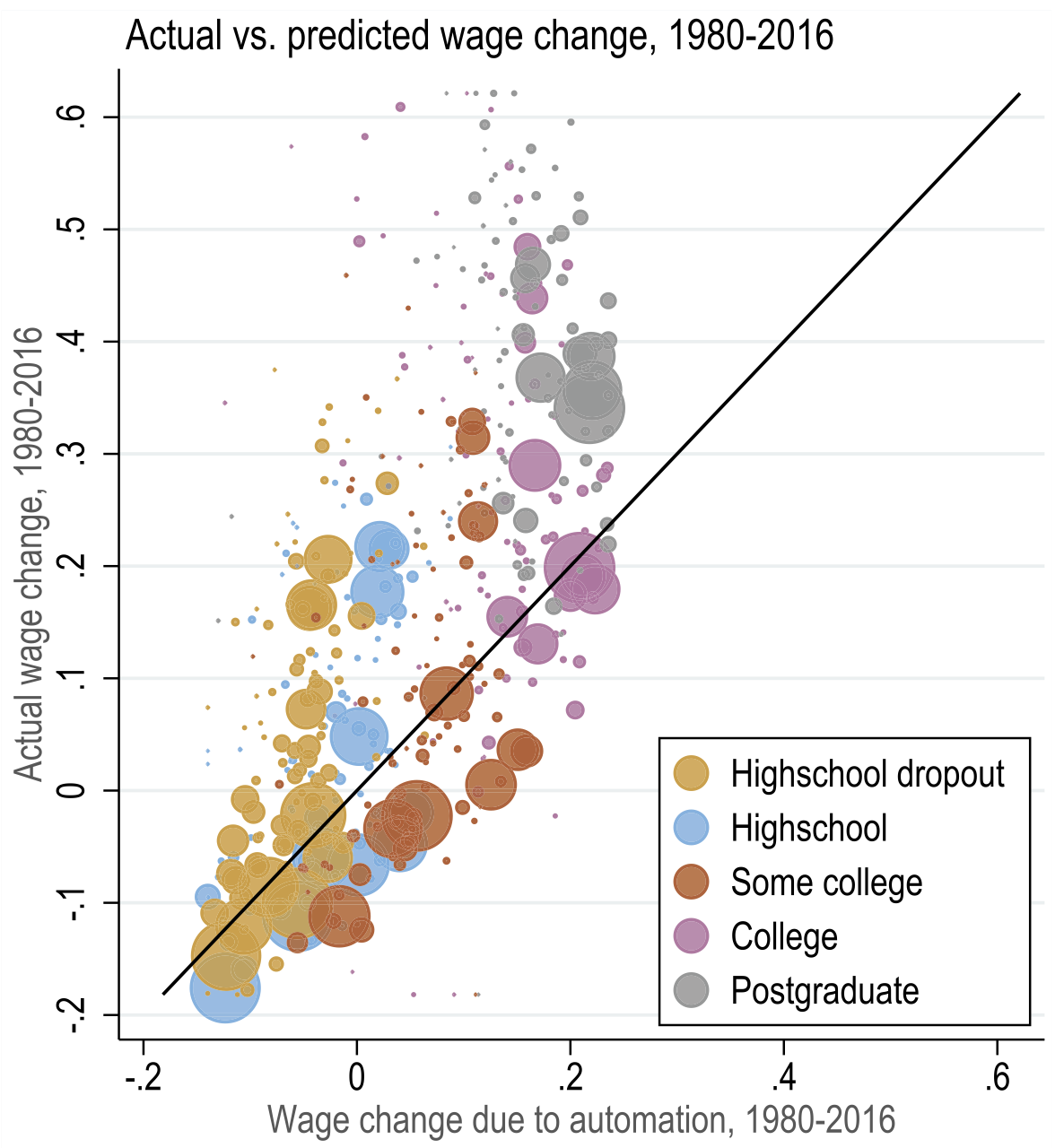
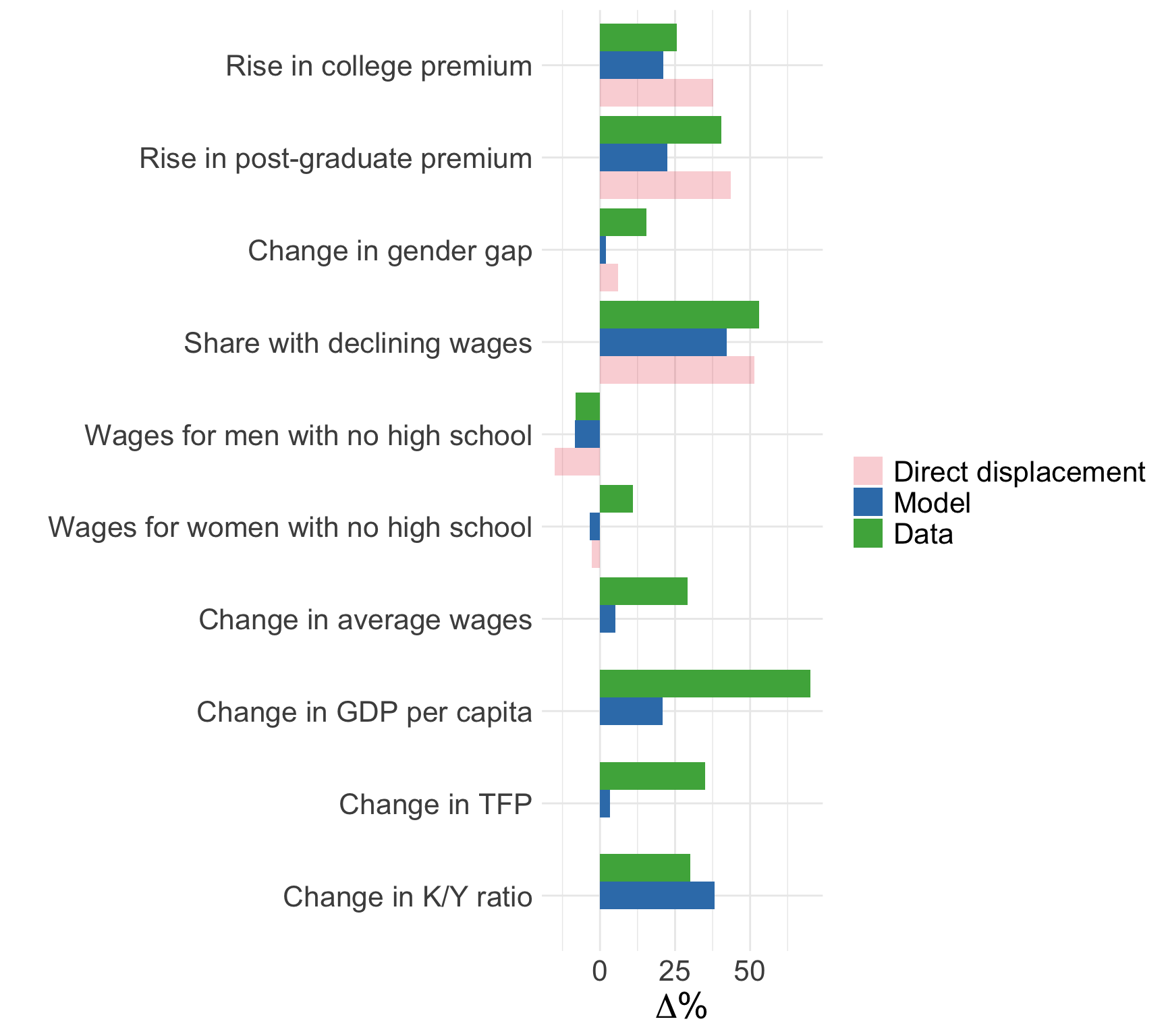
• The model has close fit to the data everywhere except top of growth distribution

  • Technology-labour complementarity at the top

  • Different kinds of jobs (winner-takes-it-all)

  • Both absent from the model

• It also predicts well changes in college premium and wages of men without high school

• But it misses big on aggregate things like GDP and TFP

  • could indicate there were factor-augmenting tech shifts, productivity deepenings, or even new tasks

  • this wold affect wage levels, but would have little impact on inequality because have shown that inequality is largely attributed to automation

• It also suggests that automation-induced investments in the model are in line with data

• It also misses on wages of women, which could suggest that supply side ignored so far can also play an important role.

Summary

Two theories linking technological advancements and labour markets

• Canonical model (SBTC)

  • Simple application of two-factor labour demand theory
  • Empirically attractive characterization of between-group inequality
  • Fails to account for within-group inequality, polarization, and displacement

• Task-based model (automation)

  • Rich model linking skills to tasks to output
  • Explains large share of changes in the wage structure since 1980s

Next lecture: Labour market discrimination on 22 Sep

Also mention that work continues because

• adoption is itself an endogenous decision

• creation of new tasks

• labour supply adjustments

Appendix: derivation of wage equations

The firm problem is to choose entire schedules ${(l(i),m(i),h(i))}_{i=0}^1$ to

$$\underset{{(l(i),m(i),h(i))}_{i=0}^1}{max}PY-w_{L}L-w_{M}M-w_{H}H$$

We normalised $P=1$. Consider FOC wrt $l(i)$:

$$\frac{Y}{y(i)}{A}_L{\alpha }_L(i)=w_L,\mathrm{\forall }i\in [0,I_L]$$

In equilibrium, all $L$-type workers must be paid same amount $\Rightarrow$

$$p(i)A_L{\alpha }_L(i)=w_L,\mathrm{\forall }i\in [0,I_L]$$

Similar argument for $w_M$ and $w_H$.

Let’s write out the profit-maximisation problem (already taking-into account $P=1$ normalisation)

$$\underset{{(l(i),m(i),h(i))}_{i=0}^1}{max}\exp ({\int }_0^1\ln y(i)\text{d}i)-w_L{\int }_0^{1}l(i)\text{d}i-w_M{\int }_0^{1}m(i)\text{d}i-w_H{\int }_0^{1}h(i)\text{d}i$$

Take the first-order derivative with respect to $l(i)$:

$$\exp ({\int }_0^1\ln y(i)\text{d}i){\int }_0^1\frac{1}{y(s)}\frac{\partial y(s)}{\partial l(i)}\text{d}s-w_L{\int }_0^1\frac{\partial l(s)}{\partial l(i)}\text{d}i=0,\mathrm{\forall }i\in [0,I_L]$$

We can substitute the expression for $\frac{\partial y(i)}{\partial l(i)}$:

$$Y\frac{A_L{\alpha }_L(i)}{y(i)}=w_L,\mathrm{\forall }i\in [0,I_L]$$

Now, imagine that marginal productivity of $L$-type worker varies across $i\in [0,I_L]$. Then, there are some tasks in this low range such that firm would make losses or positive profits. Since we assumed perfect competition, then firms would set wages at the level of tasks and there would be tasks that pay less than $w_L$, and some that pay more. This situation is unsustainable because then no $L$-type worker would supply her labour to tasks that pay lower wages and firms would not have anyone to perform the full range of tasks necessary to produce output $Y$. Therefore, all $L$-type workers earn the same wage $w_L$ which is equal to its marginal revenue.

Hence,

$$w_L=p(i)A_L{\alpha }_L(i),\mathrm{\forall }i\in [0,I_L]$$

Notice that for any two tasks $i,i^{\prime }\in [0,I_L]$, the task productivities may not be equal ${\alpha }_L(i)\ne {\alpha }_L(i^{\prime })$. The task prices $p(i),p(i^{\prime })$, therefore, need to be determined endogenously such that the equality holds ($p(i)=\frac{Y}{y(i)}$). Our normalisation of the final output price implies $\exp ({\int }_0^1\ln p(i)\text{d}i)=1$.

Similar arguments for wages of $M$-type and $H$-type workers.

$$\begin{array}{rlr}{w}_M& =p(i)A_M{\alpha }_M(i),\mathrm{\forall }i\in (I_L,I_H]w_H& =p(i)A_H{\alpha }_H(i),\mathrm{\forall }i\in (I_H,1]\end{array}$$

Appendix: derivation of skill allocations

Given the law of one price (wage) we can also write that

$$p(i){\alpha }_L(i)l(i)=p\left(i^{\prime }\right){\alpha }_L\left(i^{\prime }\right)l\left(i^{\prime }\right),\mathrm{\forall }i,i^{\prime }\in [0,I_L]$$

Given the Appendix: derivation of wage equations, it implies that

$$l(i)=l\left(i^{\prime }\right)=l,\mathrm{\forall }i,i^{\prime }\in [0,I_L]$$

Plug it into the market clearing condition for $L$

$$L={\int }_0^{I_L}l(i)\text{d}i=l\cdot I_L⟹l(i)=l=\frac{L}{I_L},\mathrm{\forall }i\in [0,I_L]$$

Similar argument for $m(i)=\frac{M}{I_H-I_L}$ and $h(i)=\frac{H}{1-I_H}$.

We have concluded above that for any task $i\in [0,I_L]$, $p(i)$ is determined such that marginal cost of $L$-type worker is equal to her marginal revenue. Notice that since same logic holds for all other tasks too, the relationship $\frac{Y}{y(i)}=p(i)$ holds for all $i\in [0,1]$. We can rewrite this

$$Y=y(i)p(i)=y\left(i^{\prime }\right)p\left(i^{\prime }\right)=Y,\mathrm{\forall }i,i^{\prime }\in [0,1]$$

Let’s consider again the set of tasks given to $L$-type workers.

$$p(i)A_L{\alpha }_L(i)l(i)=p\left(i^{\prime }\right)A_L{\alpha }_L\left(i^{\prime }\right)l\left(i^{\prime }\right),\mathrm{\forall }i,i^{\prime }\in [0,I_L]$$

Rewrite it

$$w_{L}l(i)=w_{L}l\left(i^{\prime }\right),\mathrm{\forall }i,i^{\prime }\in [0,I_L]$$

Therefore, the $L$-type workers are allocated uniformly across tasks $i\in [0,I_L]$. Let $l(i)=l,\mathrm{\forall }i\in [0,I_L]$. Then, using the market clearing condition for $L$-type workers we can write

$$l(i)=l=\frac{L}{I_L},\mathrm{\forall }i\in [0,I_L]$$

References

Acemoglu, Daron, and David Autor. 2011. “Chapter 12 - Skills, Tasks and Technologies: Implications for Employment and Earnings.” In Handbook of Labor Economics, edited by David Card and Orley Ashenfelter, 4:1043–1171. Elsevier. https://doi.org/10.1016/S0169-7218(11)02410-5.

Acemoglu, Daron, and Pascual Restrepo. 2018. “The Race Between Man and Machine: Implications of Technology for Growth, Factor Shares, and Employment.” American Economic Review 108 (6): 1488–1542. https://doi.org/10.1257/aer.20160696.

———. 2022. “Tasks, Automation, and the Rise in U.S. Wage Inequality.” Econometrica 90 (5): 1973–2016. https://doi.org/10.3982/ECTA19815.

Autor, David H. 2019. “Work of the Past, Work of the Future.” AEA Papers and Proceedings 109 (May): 1–32. https://doi.org/10.1257/pandp.20191110.

Autor, David H., Frank Levy, and Richard J. Murnane. 2003. “The Skill Content of Recent Technological Change: An Empirical Exploration*.” The Quarterly Journal of Economics 118 (4): 1279–1333. https://doi.org/10.1162/003355303322552801.

Katz, Lawrence F., and Kevin M. Murphy. 1992. “Changes in Relative Wages, 1963-1987: Supply and Demand Factors.” The Quarterly Journal of Economics 107 (1): 35–78. https://doi.org/10.2307/2118323.

Footnotes

1. For the discussion of this point, see section 3.4 in Acemoglu and Autor (2011)