7. Education Quality

KAT.TAL.322 Advanced Course in Labour Economics

Education quality

Knowledge/productivity doesn’t rise linearly with years of education.

Production process that takes inputs and develops skills.

As already mentioned in the last lecture, education in itself is produced by many factors. We’ve already mentioned innate ability, parental investments, formal schooling, etc.

In this lecture we will look closely at the education production function and study the responsiveness of education to different inputs.

We will also talk a little about how to measure output of education production function. We have already touched upon this last lecture when discussing the difference between years of education at different stages or qualifications.

Stylised facts

Education quantity vs quality

Source: World Bank

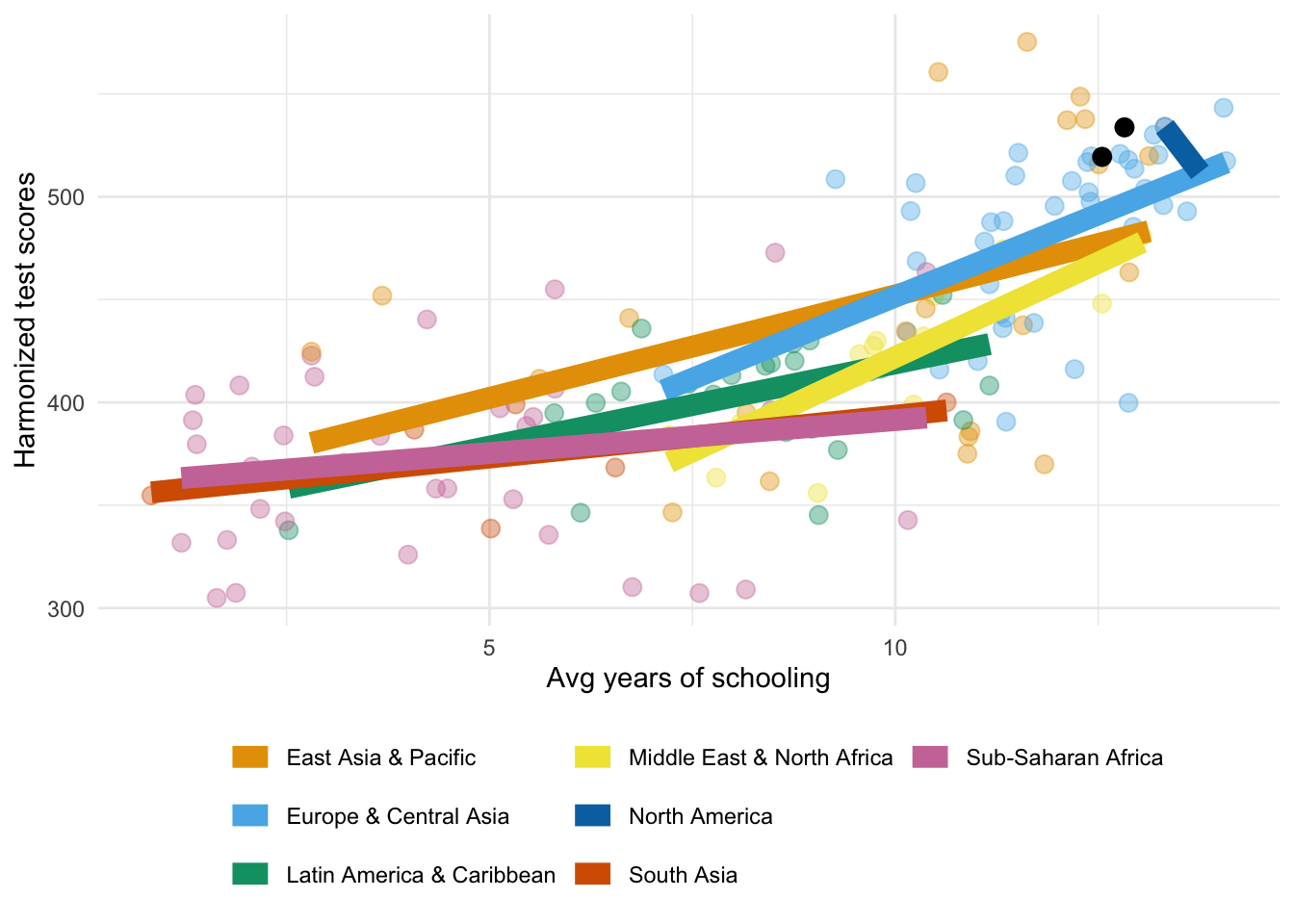
The figure above provides motivation for us to study even education production function. It shows average scores of students in standardised tests by amount of education the students have completed in each country.

To an extent that we believe that test scores do measure learning output of students, it is clear that an extra year of school doesn’t add same amount to test scores at low and high levels of education.

It can also vary between countries - a year of school in one country may produce different knowledge than year of school in another country. The two black dots in the figure are for Sweden and Finland. And we can see that between Sweden and Finland it seems that correlation between test scores and years of school is higher than on average in Europe.

Education production function

Education production function

Simple framework

Education output of pupil $i$ in school $j$ in community $k$

$$q_{ijk}=q(P_i,S_{ij},C_{ik})$$

where $\begin{array}{rl}{P}_i& \text{are pupil characteristics}\\ S_{ij}& \text{are school inputs}\\ C_{ik}& \text{are non-school inputs}\end{array}$

Let’s start from a very general framework that can help us think about education production function.

Let $q(\cdot )$ be the education production function. It accepts some inputs and produces some output.

We can allow the production function to depend on students’ own characteristics $P_i$. These can include innate ability, and can also be family characteristics of student $i$. We also allow the output to depend on school inputs $S_{ij}$. Notice that we allow the school inputs to interact with student characteristics. So, this could for example allow a researcher to study the quality of the match between specialised schools and certain group of students. Finally, we also want to allow the production to depend on some non-school inputs $C_{ik}$. We will see some examples of what these inputs can be on the next slide.

Therefore, the output of this production is that student $i$ that attended school $j$ and was subject to $k$ community gets $q_{ijk}$ education.

You will notice that the structure of this lecture is a little different from other lectures. We will start basically right away with empirical studies and will not spend that much time studying analytical predictions of a model. Couple of reasons for this. First, any of these inptus are multi-dimensional, so to develop this general production function further we would need to make a lot of assumption. Typically, people focus on one specific input and write a smaller model for that purpose. Second, it can be difficult to think about prices of these inputs. How do you price genetic makeup of a person or composition of peers.

Education production function

Measures

Output

Years of schooling, standardised test scores, noncognitive skills

Student inputs

Effort, patience, genetics, parental characteristics, family income, family size

School inputs

Teacher characteristics, class sizes, teacher-student ratio, school expenditures, school facilities

Non-school inputs

Peers, local economic conditions, national curricula, regulations, certification rules

As already mentioned in this and previous lectures, the output of human capital production function can have multiple dimensions. The simplest is, of course, to have some simple measure of years of education or highest qualification categories. However, in some studies you might want to consider more granular measures such as test scores, high-school grades or bundles of skills (cognitive/non-cognitive).

Student inputs would include all characteristics that a given student possesses. This may include characteristics of students themselves - like their effort, patience, genetics - as well as characteristics of their families - such as parents’ income, their education, characteristics of their siblings. Also note that $P_i$ may include past outcomes of the students. Remember how in the previous lecture we said that learning new skills might be easier when you already have high levels of human capital. It is the same idea.

School inputs include every resource that school can provide its children. It may be quality of their teachers, teacher-student ratios, quality of facilities, availability of specific programs, etc

Finally, non-school inputs can include all other relevant factors. For example, it can be composition of peers in the classroom (whether students are exposed to other students from similar or different backgrounds), local economic conditions (for example, if there is a recession while the child is actively developing her skills), higher level regulations (for example, any changes in school curricula, rules about attendance, etc) or certification rules for various occupations that shape a specific education track.

As you can see, you can think of many relevant inputs and many relevant outputs. So, the modelling of production function will depend on the objectives of a given research question.

Education production function

Todd and Wolpin (2003)

Achievement of student $i$ in family $j$ at age $a$

$$q_{ija}=q_a({\mathbf{F}}_{ij}(a),{\mathbf{S}}_{ij}(a),{\mu }_{ij0},{\epsilon }_{ija})$$

${\mathbf{F}}_{ij}(a)$ history of family inputs up to age $a$

${\mathbf{S}}_{ij}(a)$ history of school inputs up to age $a$

${\mu }_{ij0}$ initial skill endowment

${\epsilon }_{ija}$ measurement error in output

$q_a(\cdot )$ age-dependent production function

Todd and Wolpin (2003) provide somewhat simpler, but still general, framework to study various family- and school-inputs in education production function. Their framework is especially useful in guiding empirical work or assessing other empirical estimates.

Notice the following features of the model:

• the production function is allowed to be age-specific

  This means that similar levels of inputs can contribute differently to output at different ages. For example, maybe €50 worth of books at age 5 might mean a lot of valuable resources, but €50 worth of books at age 15 might not be so influential.

• the inputs may themselves be entire histories up to a given age $a$

  For example, if we are studying school grades at age 5, they can depend on all resources the child received since birth up to age 5; when we study grades at age 16 - all resources from birth to age 16.

This framework nests various common approaches used in the early literature with observational data. We will consider them in the next slides.

Education production function

Todd and Wolpin (2003): Contemporaneous specification

$$q_{ija}=q_a(F_{ija},S_{ija})+{\nu }_{ija}$$

Strong assumptions:

1. Only current inputs are relevant OR inputs are stable over time
2. Inputs are uncorrelated with ${\mu }_{ij0}$ or ${\epsilon }_{ija}$

First approach is contemporaneous. This is most common framework used by earliest papers, mainly dictated by data availability. Typically, early datasets were single cross-sections of children with only contemporaneous information on their families and schools.

This means that instead of full histories up to age $a$, the inputs are now simply $F_{ija}$ and $S_{ija}$. It also means that we cannot control for initial skill endowment ${\mu }_{ij0}$, which instead is now part of the error term ${\nu }_{ija}$!

It is easy to see that by adopting this kind of empirical specification we are implicitly making very strong assumptions. It is nearly impossible to defend the claims that

• only current inputs are relevant for current outputs (in some countries, attending certain kindergarten increases chances of attending better schools, attending certain schools increases chances of attending top universities), or
• that inputs are stable over time (clearly, family income can change over time, school funding can change over time), and
• that inputs are uncorrelated with the error term (which now includes ${\mu }_{ij0}$ and you can imagine that parents and schools may invest different into children with different skills).

Education production function

Todd and Wolpin (2003): Value-added specification

$$q_{ija}=q_a(F_{ija},S_{ija},q_{a-1}[F_{ij}(a-1),S_{ij}(a-1),{\mu }_{ij0},{\epsilon }_{ij,a-1}],{\epsilon }_{ija})$$

Typical empirical estimation assumes linear separability and $q_a(\cdot )=q(\cdot )$:

$$q_{ija}=F_{ija}{\alpha }_F+S_{ija}{\alpha }_S+\gamma q_{ij,a-1}+{\nu }_{ija}$$

Additional assumptions implied:

1. Past input effects decay at the same rate $\gamma$
2. Shocks ${\epsilon }_{ija}$ are serially correlated with persistence $\gamma$

Over time quality of data improved and longitudinal data became more prevalent. However, having sufficiently long follow-up period can be a struggle even nowadays. For example, in UK there are several cohort studies that were initiated since 1957 that measured various children and family outcomes at specific ages of children (at birth, age 5, age 10, etc). So, in the environment where we have few observations per child, we can look on value-added version of the model. That is, imagine we have a snapshot of children at age 5 and age 10. We can measure the change in outcomes as well as change in inputs between these two periods to try to infer model parameters.

To see it in the framework of Todd and Wolpin (2003), assume for simplicity that we have two time periods per child $a$ and $a-1$. Now, we say that output $q_{ija}$ depends on contemporaneous inputs $F_{ija}$ and $S_{ija}$ as well as past output $q_{a-1}(F_{ij}(a-1),S_{ij}(a-1))$. Notice a slight change in notation: the past output is allowed to depend on the entire history of inputs up to $a-1$, even though we still may not observe them! This is relevant for many datasets that may not record history of inputs (even nowadays, some datasets only record family income once at a certain age), but do have repeated measurements of child outcomes (for example, test scores or school grades).

Assume a very simple linear production function with full histories

$$q_{ija}=X_{ija}{\alpha }_1+X_{ij,a-1}{\alpha }_2+\dots +X_{ij1}{\alpha }_a+{\beta }_a{\mu }_{ij0}+{\epsilon }_{ija}$$

Furthermore, we assume that functional form of $q_a(\cdot )$ is same across all ages. Then, same equation at $a-1$ (already multiplied by $\gamma$) is

$$\gamma q_{ij,a-1}=\gamma X_{ij,a-1}{\alpha }_1+\dots +\gamma X_{ij1}{\alpha }_{a-1}+\gamma {\beta }_{a-1}{\mu }_{ij0}+\gamma {\epsilon }_{ij,a-1}$$

The difference (or value added) is

$$q_{ija}-\gamma q_{ij,a-1}=X_{ija}{\alpha }_1+X_{ij,a-1}({\alpha }_2-\gamma {\alpha }_1)+\dots +X_{ij1}({\alpha }_a-\gamma {\alpha }_{a-1})+({\beta }_a-\gamma {\beta }_{a-1}){\mu }_{ij0}+{\epsilon }_{ija}-\gamma {\epsilon }_{ij,a-1}$$

Therefore, it is clear that for this expression to be equivalent to the above regression equation, the following should hold

$$\begin{array}{rl}{\alpha }_v& =\gamma {\alpha }_{v-1}\\ {\beta }_v& =\gamma {\beta }_{v-1}\end{array},\mathrm{\forall }v\in 1,\dots ,A$$

In this case, all terms multiplied by ${\alpha }_a-\gamma {\alpha }_{a-1}$ and ${\beta }_a-\gamma {\beta }_{a-1}$ will disappear and we will get exactly the regression equation on the slide.

$$q_{ija}-\gamma q_{ij,a-1}=X_{ija}{\alpha }_1+{\epsilon }_{ija}-\gamma {\epsilon }_{ij,a-1}$$

In addition, it also highlights that the regression error term ${\nu }_{ija}={\epsilon }_{ija}-\gamma {\epsilon }_{ij,a-1}$. So, consistent estimation requires that ${\epsilon }_{ija}$ is serially correlated with persistence exactly equal to $\gamma$. In that case ${\nu }_{ija}$ is white noise and uncorrelated with $q_{ij,a-1}$.

If any of these assumptions don’t hold, then estimates will be biased!

Education production function

Todd and Wolpin (2003): Cumulative specification

Still assume linear separability:

$$q_{ija}=\sum _{t=1}^a{X}_{ijt}{\alpha }_{a-t+1}^a+{\beta }_a{\mu }_{ij0}+{\epsilon }_{ij}(a)$$

Estimation strategies:

1. Within-child: $q_{ija}-q_{ij{a}^{\prime }}$ for ages $a$ and $a^{\prime }$
2. Within-family: $q_{ija}-q_{i^{\prime }ja}$ for siblings $i$ and $i^{\prime }$

Each with their own caveats

Modern datasets may give us access to long histories of both inputs and outputs. So, we might think that we are finally able to estimate the parameters of the production function in a flexible way.

If there are many family and school-level characteristics in $F_{ij}(a)$ and $S_{ij}(a)$, then estimating a very flexible specification with many interaction terms might be hard to interpret. Therefore, we still have to make some simplifying assumptions. In particular, that the production is linearly separable, perhaps with only few interaction terms.

The specification still includes the potentially unobserved initial skill endowments ${\mu }_{ij0}$. But because we now have a rich longitudinal data, we could use different methods to difference it out.

First approach is to use multiple observations per child - a within-child design.

• However, if you explicitly write down the expression for $q_{ija}-q_{ij{a}^{\prime }}$, you will see that unless ${\beta }_a=\beta ,\mathrm{\forall }a$ the unobserved heterogeneity term ${\mu }_{ij0}$ will not disappear! This assumption may in fact be violated. For example, we can imagine that learning of a 2-year-old child may depend a lot more strongly on her initial skill endowment than her academic performance at 17 years old.
• Also notice that the error term in general depends on the entire history of ${\epsilon }_{ij}(a)$. This means that the estimation implicitly assumes that input choices at any age $a$ are not correlated with past, contemporaneous or future outcomes! This assumption too can be easily violated if parents or schools adjust their investments depending on past performance of students. For example, if a student does very well in one year, the school might offer additional learning materials to her next year.

Second approach is within-family design that exploits variation between siblings. However, this approach also makes some pretty strong assumptions about the production process.

• If you explicitly write down the expression for $q_{ija}-q_{i^{\prime }ja}$, you will notice that it will depend on ${\mu }_{ij0}-{\mu }_{i^{\prime }j0}$. This term will only be equal to zero if and only if we assume that only family characteristics matter for the production process and children’s own unobserved characteristics do not matter. This is very hard-to-defend assumption!

• In addition, the error term will be ${\epsilon }_{ij}(a)-{\epsilon }_{i^{\prime }j}(a)$ and all the regressors are implicitly assumed to be uncorrelated with it. This means that outcomes of one sibling cannot affect directly investments made to another sibling. This assumption can also be contested.

All in all, estimating human capital production function parameters is really hard in observational data!

Early estimates of school inputs (prior to 1995)

“resources are not closely related to student performance” (Hanushek 2003)

Source: Hanushek (2003), Table 3

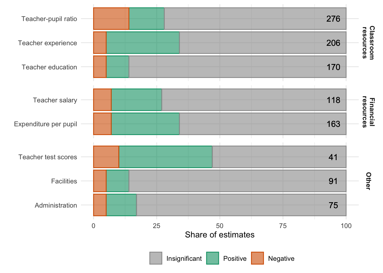
The figure above is based on the literature survey by Hanushek (2003). It shows share of reviewed papers with statistically insignificant, significant positive and significant negative effects of different types of school resources

As you can see the majority of reviewed papers find insignificant relationship between various classroom, financial and other resources available through schools on student performance. And among papers that do find significant results some are negative and others are positive. Moreover, upon closer inspection of their methodologies Hanushek (2003) concludes that papers with less robust empirical strategies find strongest effects.

Most of these papers are based on contemporaneous design in cross-sectional datasets. Table 5 in Hanushek (2003) reports similar statistics among papers that use value-added specification. But the share of insignificant findings is roughly comparable, if not somewhat higher, to the overall picture shown above. And we have seen that all specifications suffer from some kind of endogeneity.

Education production function

Non-experimental estimations

• Require strong assumptions

  • Some can be relaxed

• Require rich data

• Endogenous allocation of resources

Quasi-experimental estimations

• May not recover structural parameters

• Ignore general equilibrium

• Issues with scaling List (2022)

Summarising the discussion above, estimation of production function parameters from observational data can impose very strong assumptions on the underlying model. These assumptions most likely are violated in real data. Especially, because investments from parents and schools can endogenously react to each other as well as children’s own characteristics and past results.

Typically, to solve endogeneity issues we turn to quasi-experimental designs. However, Todd and Wolpin (2003) warn that these results too may not be sufficient to uncover the structural parameters of the production function. To make it explicit, these designs do help identify causal effects of any policies that generate the exogenous variation. Therefore, they are invaluable for policy discussions and evaluation. However, the policy changes to school inputs, for example, can also induce parents to change their investments. Therefore, causal effect of policy may not necessarily be the same as causal effect of certain inputs.

In addition to this, even if we find strong and robust causal effect in some experimental or quasi-experimental design, implementing them at larger scale might not produce similar results (List 2022). This argument is applicable not only to empirical literature on education quality, but to many other fields too. Suppose that you design an experiment and send the best of the best teacher to a remote school in Finland and find strong and positive effects on achievement of students. You conclude from this that teacher quality plays a tremendous role in education production function. But if you want to now scale it up to the entire country, where do you find thousands of teachers of exactly same quality? Even if training of would-be teachers improves as a result, there necessarily will be a distribution of teachers with different qualities. So, the impact on students may be smaller than the one identified in the causal paper.

(Quasi-)Experimental estimations

Productivity of student inputs

Student inputs: nature vs nurture

Twin models (ACDE)

Source: Neale and Maes (2004)

Twin studies are often used to study the importance of family environment and students innate bundle of skills for human capital outcomes.

Suppose we observe a pair of twins with observed outcomes $P_1$ and $P_2$. Let each twin’s outcome depend on a number of potentially unobserved (latent) factors.

• Additive genetic effects $A$

  Imagine you have information about two genes, $g_1$ and $g_2$, for all individuals. Their additive effect is, essentially, a weighted sum ${\beta }_1{g}_1+{\beta }_2{g}_2$. So, if you have $g_1=1$ then your outcome increases by ${\beta }_1$ units. If, on top of it, you have $g_2=1$, your overall outcome increases by ${\beta }_1+{\beta }_2$.

• Non-additive genetic effects $D$

  This part allows other non-linear effect of genes on outcomes. For example, there may be interactions between $g_1$ and $g_2$. In that case, if both $g_1=1$ and $g_2=1$, then your outcome would increase by ${\beta }_1+{\beta }_2+{\beta }_3$. Alternatively, it can also capture the effects of dominant genes. If you remember the classical example of dominant traits in Mendel’s experiments with pea plants, you inherit genes roughly equally from your mother and father. If either of them pass on a dominant allele to you, then your outcome will be completely determined by the dominant allele, and presence of recessive allele does not impact your outcomes in any way.

• Common environment $C$

  Every non-genetic factor that twins share such as family, common friend groups, etc.

• Idiosyncratic environment $E$

  Some other environmental factors that are uncorrelated between twins. For example, imagine that one of the twins was randomly selected to participate in some special course. Then, only one of the twins gets to experience the learning on that course, interact with peers on that course, etc.

For simplicity, we can assume that each of these unobserved factors have unit variance, although this can be easily relaxed.

We can impose some limitations on the correlations between latent factors of the twins dictated by laws of genetic inheritance and assumptions on environment.

1. Depending on the type of twins we can predict their genetic correlations.
   • Monozygotic twins have completely identical genotypes. Therefore, their genetic correlation is equal to 100% for both additive $A$ and non-additive $D$ factors.
   • Dizygotic twins share roughly 50% of their genotypes. This means the predicted correlation between additive factors $A_1$ and $A_2$ is also 50%, and correlation between non-additive factors $D_1$ and $D_2$ is 25%.
2. We assumed that environment can be split into shared and idiosyncratic. These assumptions imply $\text{Corr}(C_1,C_2)=1$ and $\text{Corr}(E_1,E_2)=0$.

Notice the lower- and upper-case letters in the diagram above. The upper-case letters denote the unobserved factors, and the lower-case letters capture the importance of these latent factors for the realised outcomes $P_1$ and $P_2$. Notice also that we assume that importance of $A_1$ for $P_1$ is same as $A_2$ for $P_2$. Basically, we are saying that each twin benefits from different factors in the same way, which seems a reasonable assumption.

However, a stronger assumption we are making is that genetic effects $A$ and $D$ are uncorrelated with environmental factors $C$ and $E$. This is a very strong assumption and can be easily refuted in many settings (see, for example, Barcellos, Carvalho, and Turley 2018; Arold, Hufe, and Stoeckli forthcoming).

Given these assumptions and that , the objective is to find coefficients $\{a,c,d,e\}$ that are consistent with observed variance-covariance matrices of outcomes between twins. In particular, the system of equations can be written as

$$\begin{array}{rl}\text{Var}(P_i)& =a^2+d^2+c^2+e^2\\ {\text{Cov}}_{MZ}(P_1,P_2)& =a^2+d^2+c^2\\ {\text{Cov}}_{DZ}(P_1,P_2)& =\frac{1}{2}{a}^2+\frac{1}{4}{d}^2+c^2\end{array}$$

A useful statistic often used in these kinds of studies is heritability estimator

$$h^2=\frac{a^2+d^2}{\text{Var}\left(P_i\right)}$$

You probably have noticed that the above system has 3 equations with 4 unknowns. This means that the system is underidentified and we need to impose another restriction to be able to estimate it. Often, the choice is between ACE and DCE models. So, if we choose ACE model, we assume implicitly that $d=0$.

Student inputs: nature vs nurture

Twin models: Polderman et al. (2015)

Meta-analysis of >17,000 twin-analyses (>1,500 cognitive traits)

• 47% of variation due to genetic factors
• 18% of variation due to shared environment

Adoption studies

Fagereng, Mogstad, and Rønning (2021): Korean Norwegian

• Wealth: $a^2\approx 58$% and $c^2\approx 37$%
• Education: $a^2\approx 49$% and $c^2\approx 6$%

Sacerdote (2007): Korean American

• College: $a^2\approx 41$% and $c^2\approx 16$%

Polderman et al. (2015) surveys more than 2 700 publications that exploit twin models to study more than 17 000 different outcomes, including more than 1 500 cognitive traits. These could be outcome of human capital production function, and the results can provide us with some understanding of relative importance of student-specific inputs.

The results suggest that on average 47% of variation in observed cognitive outcomes can be attributed to genetic factors and around 18% of the variation - to shared environment.

However, as mentioned on the previous slide, these estimates may be biased by possible gene-environment correlations that are unaccounted for in these models. Another possible source of bias is presence of assortative mating: parents may be more genetically similar to each other than to a random person in the population. In other words, people with certain genotypes (and/or observed traits) may be more likely to form a family (Torvik et al. 2022).

To account for these potential issues, some studies exploit quasi-random assignment of adoptees to families to eliminate correlations between latent factors. The quasi-random assignment at adoption ensures zero genetic correlation between adopted and non-adopted siblings. Therefore, full correlation between their outcomes can be attributed to shared envirionment. The impact of genetic factor can then be deduced from the correlations between biological siblings. The papers find somewhat similar effects of genetic factors: between 40% and 60% depending on the outcomes. There is larger variation in shared environmental factors: from 6% to 37%.

All in all, the estimates suggest that genes and environment contribute roughly equally to the observed outcomes. This conclusion is quite attractive from the policy perspective since about half of variation in outcomes can be influenced by policies and economic incentives.

Productivity of school inputs

Productivity of school inputs

School expenditures: review by Handel and Hanushek (2023)

Exogenous variation due to court decisions or legislative action

Source: Table 10 (Handel and Hanushek 2023)

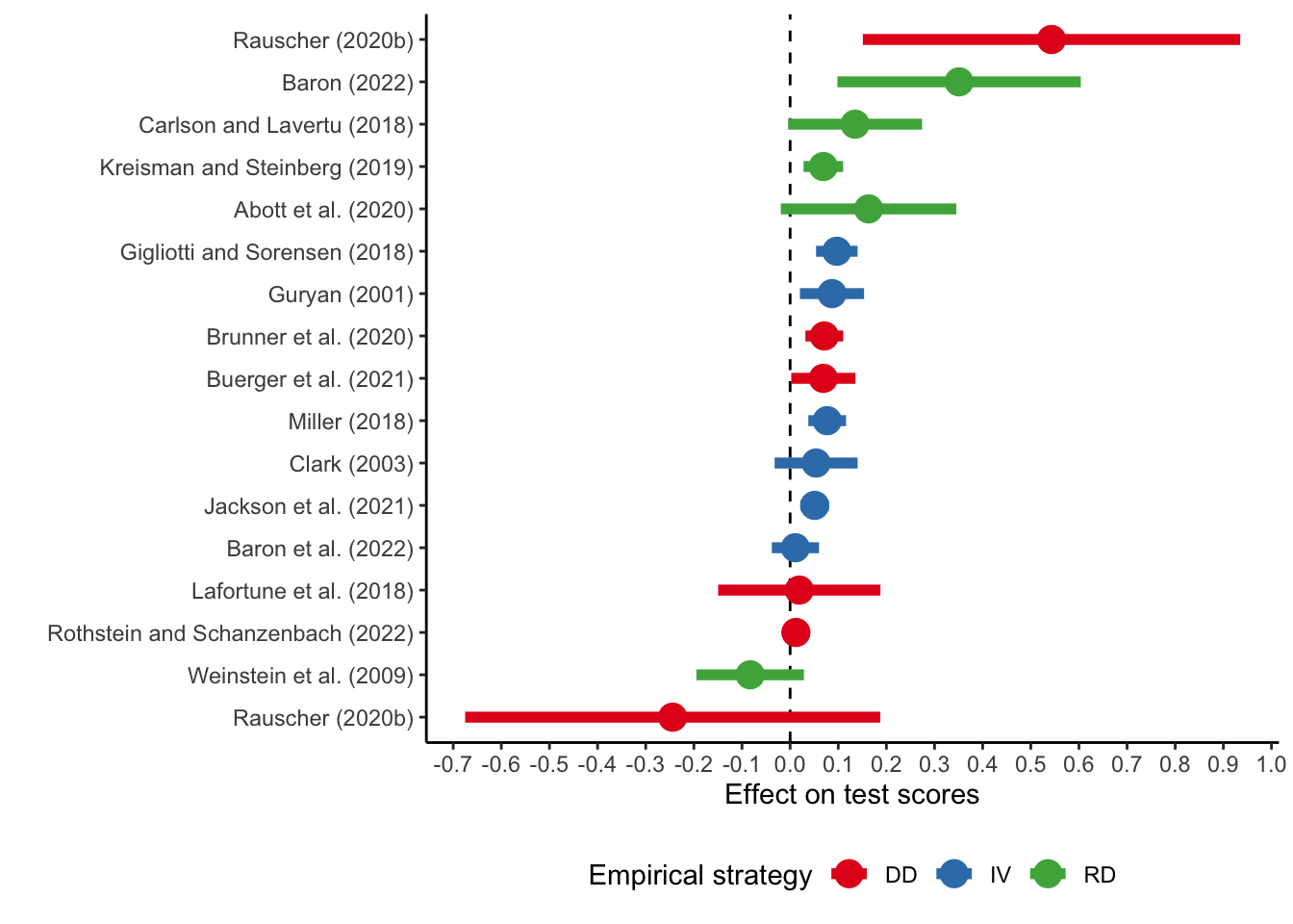
There is also quasi-experimental evidence on the productivity of various school inputs.

Here, you can see a review of papers that focus on school expenditures in general. These papers exploit exogenous variation in school expenditures due to court decisions or legislative actions in the US.

Court cases. Since 1968 there were several court cases where equity (how school funds are distributed between students) and adequacy (whether school funds are sufficient for its goals) of school funds was questioned. These cases provide plausibly exogenous changes in distribution and level of expenditures by schools.

Even though court decisions mandate changes in school funding, they typically do not provide exact numbers. After the court decision, state legislative bodies have to decide whether (i.e., they may not comply with the decision) and by how much they will change school funding. These state decisions can very well be endogenous.

Legislative actions. Even without court cases, many states have passed different bills that affect school funding (for example, Proposal A in Michigan, property tax elections, etc; see Handel and Hanushek (2023) for more info).

The figure above summarises the results on standardised test scores from various relatively recent papers. As you can see, the results vary quite a lot ranging from negative to positive, with many estimates still in the vicinity of zero. The high variation could be attributed to

• heterogeneity in different groups of students (for example, Rauscher (2020) find positive effect in rural districts in Kansas and insignificant negative effect in urban districts),
• sensitivity to data restrictions and empirical designs.

Productivity of school inputs

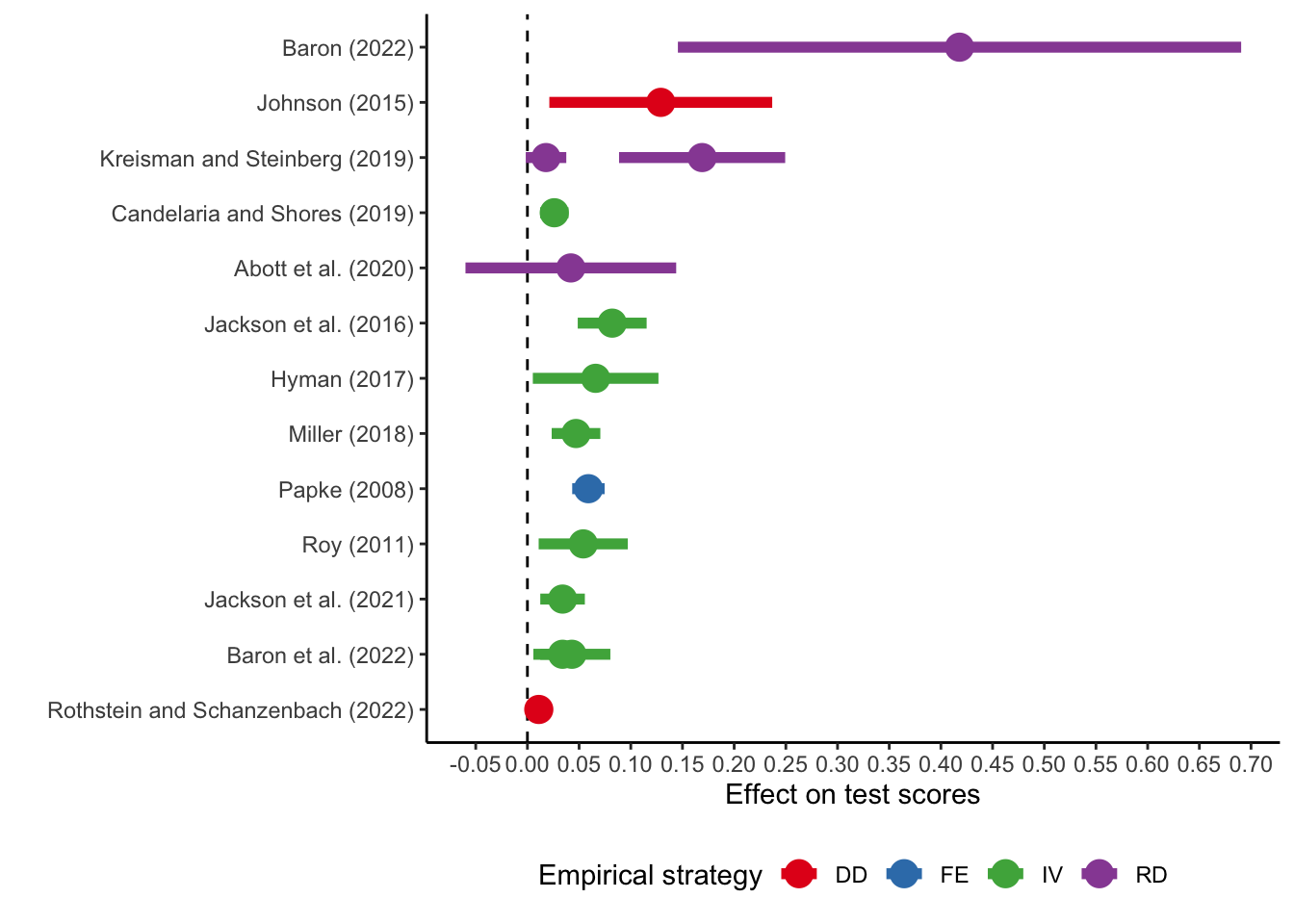
School spending: review by Handel and Hanushek (2023)

• Large variation of spending effects on test scores

• Not clear how money was used

• Role of differences in regulatory environments

• Similar results for participation rates are all positive (mostly significant)

So, even with modern methods and research designs, the overall conclusion is similar to early studies: change in school resources, or funding in particular, does not seem to affect students systematically in certain way. However, this result may not be all that interesting because simply increasing amount of funding does not necessarily tell us how the extra money is spent. So, it could be that a more targeted spending on certain resources could have a strong positive or negative impact on the production function.

Besides we can still make an argument that parental investments into children might have responded to these school funding changes as well. For example, if parents know that school now spends more money on extracurricular activities of children, they may reduce amount of family budget that is spent on these activities of children. So, even though school funding has increased, the overall amount of resources invested into children may not have changed much. This inter-dependence of investment decisions is very difficult to control for appropriately.

Finally, the choice of outcome can also play a huge role for estimates. Even though the estimates on test scores vary a lot and largely close to zero, the results on participation in various stages of education are positive and mostly significant.

Source: Table 10 (Handel and Hanushek 2023)

Productivity of school inputs

Class size: Joshua D. Angrist and Lavy (1999)

Quasi-experimental variation in Israel: Maimonides rule

Rule from Babylonian Talmud, interpreted by Maimonides in XII century:

If there are more than forty [students], two teachers must be appointed

Sharp drops in class sizes with 41, 81, … cohort sizes in schools

Regression discontinuity design (RDD)

Alternatively, there are numerous papers that study the productivity of specific school resources. One of the well-studied resources is class size, and the classical paper in this literature is Joshua D. Angrist and Lavy (1999).

One way that schools might allocate their funds is through class sizes. If they have large class sizes, then they need fewer classrooms and hire fewer teachers. But in large class sizes, a given student gets less teacher time and may be “left behind”. You can easily imagine, therefore, that schools have to find optimal class sizes that would balance the expenditures and student achievements.

Joshua D. Angrist and Lavy (1999) uses exogenous variation in class sizes in Israel due to Maimonides rule. It’s an ancient rule that states there cannot be more than 40 students per teacher. Thus, if the cohort size exceeds multiples of 40 (for example, there are 41, 81, students), then students are split into two classes of equal sizes. These sharp drops in class sizes allow the authors to use regression discontinuity design to study average achievement of students in a given cohort.

Productivity of school inputs

Class size: Joshua D. Angrist and Lavy (1999)

Source: Figure I (Joshua D. Angrist and Lavy 1999)

Productivity of school inputs

Class size: Joshua D. Angrist and Lavy (1999)

Maimonides rule: $f_{sc}=\frac{E_s}{\text{int}\left(\frac{E_s-1}{40}\right)+1}$

“Fuzzy” RDD

First stage: $n_{sc}=X_{sc}{\pi }_0+f_{sc}{\pi }_1+{\xi }_{sc}$

Second stage: $y_{sc}=X_s\beta +n_{sc}\alpha +{\eta }_s+{\mu }_c+{ϵ}_{sc}$

The rule can be written down mathematically as a function of cohort size at school $s$, $E_s$. Let it be denoted by $f_{sc}$.

You can notice in the previous figure that actual class size is consistent with the rule, but does not always follow it closely. Even when enrolment cohort size is below 40, some school must decide to split the students into two classes, since we see that average class size hovers around 30 students. Therefore, instead of sharp RDD, the authors adopt “fuzzy” RDD. Sharp RDD requires that only people on one side of the cutoff can be included in treatment group. Fuzzy RDD allows people on either side of the cutoff to be included in the treatment group; it only requires that probability of treatment jumps discontinuously around cutoff. For more discussion of the method, you can check Chapter 6 in Joshua David Angrist and Pischke (2009).

Fuzzy RDD can be estimated using IV regression. The first stage regresses participation in treatment on the eligibility rule. So, in this case, it regresses actual class size $n_{sc}$ on Maimonides rule $f_{sc}$. Then, the second stage regresses student outcome $y_{sc}$ on class size $n_{sc}$.

The authors use cross-sectional data on 4th and 5th graders in 1991. Collection of data was more sporadic back in the days and availability of good quality data on student achievements was not yet standard. In 1991 was the year when specifically the cohorts of 4th and 5th graders in Israel were given standardised tests to measure their academic achievements. The authors augment this data merging information on school characteristics and class sizes from other sources.

Productivity of school inputs

Class size

Source: Angrist and Lavy 1999

	Grade 4		Grade 5
	Reading	Math	Reading	Math
Class size	-0.150	0.023	-0.582	-0.443
	(0.128)	(0.160)	(0.181)	(0.236)
Mean score	72.5	68.7	74.5	67.0
SD score	7.8	9.1	8.2	10.2
Obs.	415	415	471	471

Source: Angrist et al. 2019

	Grade 5
	Reading	Math
Class size	-0.006	-0.062
	(0.066)	(0.088)
Mean score	72.1	68.1
SD score	17.4	20.6
Obs.	225 108	226 832

The authors report very strong negative effects of class sizes on student achievements at grade 5. The impact on students at grade 4 is negligible. Basically, increasing the class size by 10 people reduces average reading score in that class by 5.8 points (or 8% of mean score) and average math score - by 4.4 points (or 7% of mean score).

However, if you look closely at all estimation results, you will notice that they can be very sensitive to regression specification. In fact, in a second paper Joshua D. Angrist et al. (2019) replicate the research design using a larger sample of 5th graders taking the tests between 2002 and 2011. The new results show virtually zero effect of class size on student achievement. The authors attribute the differences between studies to

1. changes in the production function of education, and
2. misspecification of regression equation in Joshua D. Angrist and Lavy (1999) (Joshua D. Angrist et al. (2019) also redo the analysis in the original 1991 sample using more modern specifications and report insignificant results).

Productivity of school inputs

Class size: Krueger (1999), Chetty et al. (2011)

Project STAR: 79 schools, 6323 children in 1985-86 cohort in Tennessee

Randomly assigned students and teachers into

• small class (13-17 students)
• regular class (22-25 students)
• regular class + teacher’s aide (22-25 students)

$$Y=\alpha +{\beta }_{S}SMALL+{\beta }_{A}AIDE+X\delta +\epsilon$$

Randomization means students between classes are on average similar

$\mathbf{\Rightarrow }{\beta }_S$ and ${\beta }_A$ are causal

Another classical example studying the impact of class size on student achievements is Project STAR, a large-scale randomised experiment conducted in the US in 1985-86. The experiment randomly assigned kindergarten students and teachers within a given school to one of three class sizes with different student-to-teacher ratios. After the initial assignment, students were to remain in same classes for the next four years.

Because it is a randomised experiment, a simple regression of class size (treatment group) on student outcomes should provide causal evidence. This is essentially the empirical strategy adopted by Krueger (1999).

Nevertheless, in the field experiments (i.e., implemented in real-life setting instead of a lab) maintaining randomisation can be difficult.

• Some students who were initially part of the experiment may have moved away or repeated grades. These decisions can be endogenous and can depend on treatment assignment. Therefore, their exclusion from the data can lead to biased results.

• Some students were were not part of the initially randomised cohort could have joined the schools/classes in subsequent years (grades 1-3). These decisions, too, could be endogenous and may depend on treatment assignment status.

  Even though they were also randomly assigned to different types of classes at the point when they joined the participating schools, they were also subject to this different class size for fewer years than the original cohort. This too could change the estimated paramters.

• Some students could transfer between class types after the randomisation. This could very well be endogenous decision (maybe parents believe the other class type is more beneficial and really try to get their kid to that class). For example, children initially assigned to small classes spent on average only 2.27 years in a small class. Children initially assigned to a regular class spend 0.13 years in a small class.

Chetty et al. (2011) revisit the analysis of Krueger (1999), while trying to account for the above issues.

Productivity of school inputs

Class size

Source: Table V (Krueger 1999)

	Test scores
	Kindergarten	Grade 1	Grade 2	Grade 3
SMALL	5.370	6.370	5.260	5.240
	(1.190)	(1.110)	(1.100)	(1.040)

Source: Table V (Chetty et al. 2011)

	Test score, %	College by age 27, %	College quality, $	Wage earnings, $
SMALL	4.760	1.570	109.000	-124.000
	(0.990)	(1.070)	(92.600)	(336.000)
Avg dep var	48.67	45.5	27 115	15 912
Obs.	9 939	10 992	10 992	10 992

The original results in Krueger (1999) suggest strong and positive effect of smaller class size on average test scores of students throughout four years in primary schools.

However, the revised results in Chetty et al. (2011) show that there is a strong contemporaneous effect of smaller class size on test scores upon entry to the kindergarten. However, when the authors looked at longer-term outcomes such as college education and earnings, there is a strong zero result. That is, having been assigned to smaller classes did not affect students’ propensity to get higher education, study in better colleges or have higher earnings.

Thus, the conclusion is that class sizes can have large impact on short-term student outcomes, but eventually their effects fade out.

Productivity of school inputs

Class quality: Chetty et al. (2011)

Notice: random assignments of peers ($QUAL$)

Source: Table VIII (Chetty et al. 2011)

	Test score, %	College by age 27, %	College quality, $	Wage earnings, $
QUAL	0.662	0.108	9.328	50.610
	(0.024)	(0.053)	(4.573)	(17.450)
Obs.	9 939	10 959	10 959	10 959

In addition to the direct analysis of class size, Chetty et al. (2011) also notice that by randomly assigning students to class, the experiment also randomised the set of peers. Thus, in addition to experiencing smaller or regular class sizes, students were randomly exposed to classes of different qualities (measured by average peer scores in tests).

The above table shows the corresponding estimation results where main regressor is class quality. They suggest

• strong positive impact on test scores at $t=0$ (kindergarten), and
• very small positive effect on college education and college characteristics, but
• strong positive effect on annual wage earnings (although economic magnitude may be small).

So, these results also show the fade-out effect of the experiment on academic achievements of students. But they also suggest the impact re-emerges later in the labour market. The authors suggest that impact of peer quality on development of non-cognitive skills could explain the fade-out and re-emergence of the effect on adult earnings.

Curiosity time

Can you think of other potential channels through which peer quality could affect adult earnings decades later?

Productivity of school inputs

Class quality and noncognitive skills: Chetty et al. (2011)

Source: Table IX (Chetty et al. 2011)

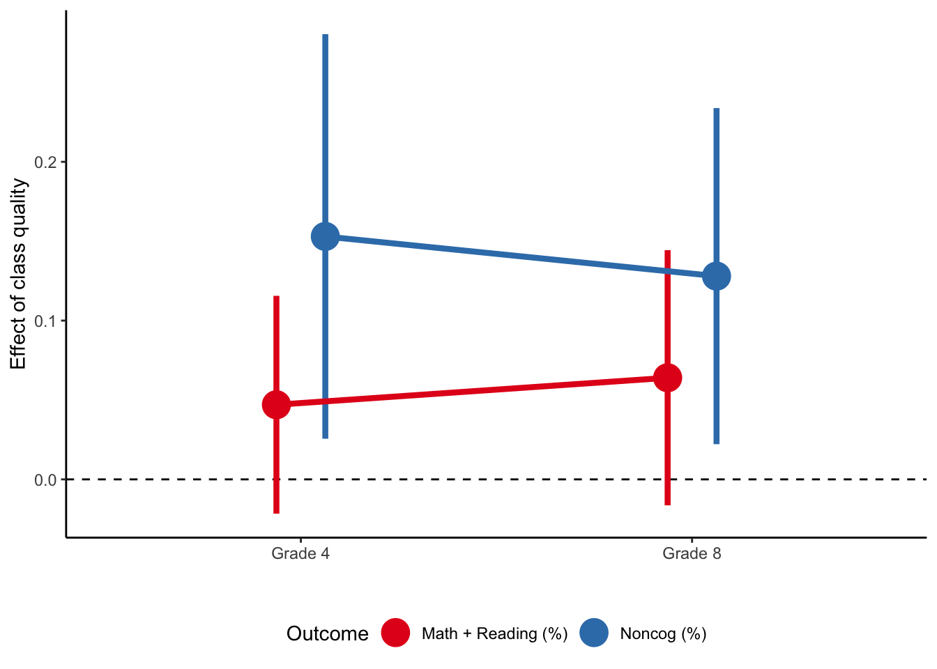
In grades 4 and 8, teachers in the participating schools were asked to evaluate a subset of students on a number of behavioural measures in four dimensions

• effort,
• initiative,
• nonparticipatory behaviour, and
• student’s value of class.

The figure above shows the results of estimations on math and reading scores (cognitive skills) and composite index based on the behavioural scores (noncognitive skills). We can easily observe that even though the impact on cognitive measures is statistically insignificant, the impact on noncognitive skills is large and positive.

Productivity of school inputs

Teacher incentives: Fryer (2013)

2-year pilot program in 2007 among lowest-performing schools in NYC

• 438 eligible schools, 233 offered treatment, 198 accepted, 163 control

• Relative rank of schools in each subscore

• Bonus sizes:

  • $3,000/teacher if 100% target
  • $1,500/teacher if 75% target

Another possible source for variation in class qualities is the quality of the teachers. Fryer (2013) investigate whether effort of teachers plays an important role in the development of students’ skills.

To answer this question they use a 2-year randomised experiment conducted in New York in 2007. They randomly selected schools in the area and offered them money for extra teacher incentives. These incentives were tied to student test scores, improvements in their scores over time and participation in the learning activities. The researchers set target achievement levels to the schools. If a school fully met the target, then it’d get $3 000/teacher $\times N$ teachers. If it only met 75% of the target, then the school would get $1 500/teacher $\times N$ teachers.

Productivity of school inputs

Teacher incentives: Fryer (2013)

Instrumental variable approach (LATE = ATT):

$$\begin{array}{rl}Y& ={\alpha }_2+{\beta }_{2}X+{\pi }_2\text{incentive}+ϵ\\ \text{incentive}& ={\alpha }_1+{\beta }_{1}X+{\pi }_1\text{treatment}+\xi \end{array}$$

Because schools were allowed to decide whether they want to participate in the program, actual status of incentive scheme is, in fact, endogenous. The only properly randomised variable is whether schools were offered the treatment or not.

For this reason, the estimation strategy cannot just be an OLS regression of student outcomes on amount of incentives received. The authors choose an IV regression, where first stage regresses amount of incentives on treatment assignment, and second stage regresses student outcomes on incentives.

As usual, the validity of this strategy requires instrument relevance, exogeneity and exclusion. The relevance of the instrument is high since 85% of schools accept invitation to participate in the program. Exogeneity assumption is also ensured by the randomisation of which schools are contacted and which are not. Exclusion restriction requires that treatment assignment only affects children’s outcomes via incentive scheme. Do you think this assumption can be violated?

Productivity of school inputs

Teacher incentives: Fryer (2013)

Source: Tables 4 and 5 (Fryer 2013)

	Elementary	Middle	High
English	-0.010 (0.015)	-0.026 (0.010)	-0.003 (0.043)
Math	-0.014 (0.018)	-0.040 (0.016)	-0.018 (0.029)

• Incentives too small and too complex
• Bonuses to schools (not teachers)
• Effort of existing teachers vs selection into teaching

The table above shows a selection of estimation results.

We can see that the incentive scheme seems to have had negative impact on students’ scores, if at all. Most of the coefficients are statistically insignificant. Only students in middle school have experienced statistically significant reduction in English and Math scores. In Table 5 in Fryer (2013) we can also see that graduation rates of students in participating schools have fallen by about 5pp.

Before we can make any general statements from these results, it is worth mentioning a few things.

• The incentive scheme may have been too small ($3 000 amounts to about 4% of annual teacher salary) and too complicated (many different activities to achieve the target). Because of these there might have been no substantial change in actual teacher effort; hence, no impact on students’ outcomes.
• Another possibility is that schools in control group (those that were not offered incentive scheme) might have adjusted their behaviour upon realising that this experiment is taking place. Maybe they wanted to compete with the treated schools thinking the treated schools would up their game.
• A critical part of the experiment is that the bonuses were paid to schools as a whole, not to teachers based on their effort. It was then up to schools to decide how to distribute this money among their teachers. They could choose to pay more to best-performing teachers or distribute money equally among all teachers. Some suggest that latter is more common, which creates a free-rider problem. In this case, any individual teacher will have even fewer incentives to change their own effort level.
• Finally, the experiment focuses on effort levels of existing teachers. It is an important question and can be of value to policy makers. However, concluding from this experiment that teachers’ effort plays no role in student outcomes and applying it to remove all requirements to teachers can be grossly misleading. The incentives in place can affect the types of people that decide to become teachers and the variation in their skills and efforts can play a big role in students’ achievements.

Productivity of school inputs

Teacher incentives: Biasi (2021)

Change in teacher pay scheme in Wisconsin in 2011:

• seniority pay (SP): collective scheme based on seniority and quals
• flexible pay (FP): bargaining with individual teachers

Main results:

• FP $\uparrow$ salary of high-quality teachers relative to low-quality

• high-quality teachers moved to FP districts (low-quality to SP)

• teacher effort $\uparrow$ in FP districts relative to SP

• student test scores $\uparrow 0.06\sigma$ (1/3 of effect of $\downarrow$ class size by 5)

Another paper by Biasi (2021) which studies the impact of monetary incentives among teachers on students’ outcomes. This time we examine the effect of changing the salary scheme from seniority pay to flexible pay. We can argue that transition to flexible pay incentivises high-quality teachers to put in more effort into their teaching since now they can be compensated accordingly. Whereas under seniority pay, the salary scheme does not depend on individual effort.

This paper shows significant positive effects of flexible pay on

• actual salaries of high-quality teachers,
• effort levels of teachers, and
• student test scores.

She also documents selective mobility of teachers: high-quality teachers prefer to move to schools with flexible pay, while lower-quality teachers move in opposite direction.

Curiosity time

Imagine now that entire state of Wisconsin, or even United States, decides to switch to flexible pay after seeing these results. Can you reason about possible effects on teachers’ wages and efforts? Try to use the models of labour supply and demand from earlier lectures. Do you think there will be changes to which people decide to become teachers?

Productivity of non-school inputs

Peer effects: Abdulkadiroğlu, Angrist, and Pathak (2014)

Admission to elite high school in Boston

Peer math scores, Figure 2 (Abdulkadiroğlu, Angrist, and Pathak 2014)

We have seen already earlier in this lecture that the composition of peers can have a lasting impact on individual outcomes.

But still many people question the role of selective schools on student outcomes. Do elite schools or universities really improve students’ skills or are they just really good at selecting best students?

Productivity of school inputs

Peer effects: Abdulkadiroğlu, Angrist, and Pathak (2014)

Source: Table VI (Abdulkadiroğlu, Angrist, and Pathak 2014)

	Parametric	Nonparametric
Attended any college	0.010	0.031
	(0.032)	(0.019)
Attended 4-year college	0.003	0.013
	(0.041)	(0.026)
Attended competitive college	-0.011	-0.004
	(0.051)	(0.029)
Attended highly competitive college	-0.009	-0.014
	(0.032)	(0.017)

So, the results suggest that at the margin of admission getting into an elite high-school does not impact further academic achievements in a significant way. Abdulkadiroğlu, Angrist, and Pathak (2014) also show no impact on test scores.

However, it is worth noting that these results may not be entirely generalisable to the rest of the population.

• Children who decide to apply to these schools in the first place might be different from the rest of population. For example, they may already be more ambitious and set on attending good universities.
• It might be that the process of preparation for admission exams is a treatment in itself. So, the process of preparation for these exams incentivises children to put more effort in further studies, irrespective of them being admitted.
• There may be an effect of attending the elite schools, but these effects may not fully show up in the outcomes considered by the authors. For example, children might be forging long-term networks that could aid them in the labour market, either as employees or as entrepreneurs. But the authors do not study the labour market outcomes and earnings. It can also be that the type of connections formed in elite schools change the preferences and opinions that might affect other behaviours, such as political participation and party affiliations. These do not necessarily impact college attendance or test scores.

Productivity of school inputs

Peer effects

Dale and Krueger (2002) study admission into selective colleges in the US

• No effect on average earnings
• $\uparrow$ earnings of students from low-income families

Kanninen, Kortelainen, and Tervonen (2023): selective schools in Finland

• $\uparrow$ university enrolment and graduation rates
• No impact on income
• Change edu preferences, not skills!

Pop-Eleches and Urquiola (2013): selective schools and tracks in Romania

• $\uparrow$ university admission exam score
• $\downarrow$ parental investments
• $\uparrow$ marginalisation and negative interactions with peers

Overall, there is little consensus on peer effects, selectivity and tracking in education. Some find positive, some find zero effects.

It is clear that these kinds of studies may be hard to generalise to the rest of the population. However, the results may also be attenuated by the process of preparing for addmissions alone.

In addition, the other papers make it also clear that being admitted to an elite college can impact children in more than one way. And it is not entirely clear that they would all work in the same direction later in the labour market and general life.

Since there is no clear consensus yet, research on these questions continues.

Productivity of non-school inputs

Productivity of non-school inputs

Curriculum: Alan, Boneva, and Ertac (2019)

RCT among schools in remote areas of Istanbul

Carefully designed curriculum promoting grit ($\ge 2$h/week for 12 weeks)

Treated students are more likely to

• set challenging goals
• exert effort to improve their skills
• accumulate more skills
• have higher standardised test scores

These effects persist 2.5 years after the intervention

The core of the experiment was to teach children the importance of their effort as opposed to their skills. The treated children were taught how to respond to difficult situations and failures, and how important setting goals is.

The authors find that treated children become more ambitious and resilient. Even more interesting that these effects were still there 2.5 years later, observed in the differences in standardised math scores.

So, Alan, Boneva, and Ertac (2019) demonstrate the importance of the ability to learn, especially from setbacks.

Productivity of non-school inputs

Curriculum: other evidence

Squicciarini (2020): adoption of technical education in France in 1870-1914

• higher resistance in religious areas, led to lower economic development

Machin and McNally (2008): ‘literacy hour’ introduced in UK in 1998/99

• highly structured framework for teaching

• $\uparrow$ English and reading skills of primary schoolchildren

Overall, it seems that the content of what is taught in the classroom is important for individuals and overall societies. It can have power to shape future development of the entire economies. There is also the idea that developing a strong curriculum at early stages of education would allow children to learn more and faster at later stages. This is consistent with skill formation theory in Cunha and Heckman (2007) where evolution of human capital depends positive on its existing stock (skills beget skills).

However, one aspect that the above studies on curricula did not explore yet is the impact on indivdiuals in the long run (for example, on their earnings, health or political behaviour).

Summary

• Academic achievement is complex function of student, parent, school and non-school inputs

• Measuring achievement can also be difficult

• Genetic and environmental factors from twin studies almost 50/50

• Large variation in school resource effects (from $\ll 0$ to $\gg 0$)

  • How resources are used?
  • Which resources are most effective?

• Studies of class size, teacher incentives, peer effects and curricula

• Another (often overlooked) step is scaling up to the population

Next lecture: Technological shift and labour markets on 17 Sep

References

Abdulkadiroğlu, Atila, Joshua Angrist, and Parag Pathak. 2014. “The Elite Illusion: Achievement Effects at Boston and New York Exam Schools.” Econometrica 82 (1): 137–96. https://doi.org/10.3982/ECTA10266.

Alan, Sule, Teodora Boneva, and Seda Ertac. 2019. “Ever Failed, Try Again, Succeed Better: Results from a Randomized Educational Intervention on Grit*.” The Quarterly Journal of Economics 134 (3): 1121–62. https://doi.org/10.1093/qje/qjz006.

Angrist, Joshua David, and Jörn-Steffen Pischke. 2009. Mostly Harmless Econometrics: An Empiricist’s Companion. Princeton: Princeton University Press.

Angrist, Joshua D., and Victor Lavy. 1999. “Using Maimonides’ Rule to Estimate the Effect of Class Size on Scholastic Achievement.” The Quarterly Journal of Economics 114 (2): 533–75. https://www.jstor.org/stable/2587016.

Angrist, Joshua D., Victor Lavy, Jetson Leder-Luis, and Adi Shany. 2019. “Maimonides’ Rule Redux.” American Economic Review: Insights 1 (3): 309–24. https://doi.org/10.1257/aeri.20180120.

Arold, Benjamin W, Paul Hufe, and Marc Stoeckli. forthcoming. “Genetic Endowments, Educational Outcomes, and the Moderating Influence of School Quality.” Journal of Political Economy: Microeconomics, forthcoming. https://www.paulhufe.net/_files/ugd/ff8cd2_0844e70fa85e409c866eb4b09f6af243.pdf.

Barcellos, Silvia H., Leandro S. Carvalho, and Patrick Turley. 2018. “Education Can Reduce Health Differences Related to Genetic Risk of Obesity.” Proceedings of the National Academy of Sciences 115 (42). https://doi.org/10.1073/pnas.1802909115.

Biasi, Barbara. 2021. “The Labor Market for Teachers Under Different Pay Schemes.” American Economic Journal: Economic Policy 13 (3): 63–102. https://doi.org/10.1257/pol.20200295.

Chetty, Raj, John N. Friedman, Nathaniel Hilger, Emmanuel Saez, Diane Whitmore Schanzenbach, and Danny Yagan. 2011. “How Does Your Kindergarten Classroom Affect Your Earnings? Evidence from Project Star *.” The Quarterly Journal of Economics 126 (4): 1593–1660. https://doi.org/10.1093/qje/qjr041.

Cunha, Flavio, and James Heckman. 2007. “The Technology of Skill Formation.” American Economic Review 97 (2): 31–47. https://doi.org/10.1257/aer.97.2.31.

Dale, Stacy Berg, and Alan B. Krueger. 2002. “Estimating the Payoff to Attending a More Selective College: An Application of Selection on Observables and Unobservables.” The Quarterly Journal of Economics 117 (4): 1491–1527. https://www.jstor.org/stable/4132484.

Fagereng, Andreas, Magne Mogstad, and Marte Rønning. 2021. “Why Do Wealthy Parents Have Wealthy Children?” Journal of Political Economy 129 (3): 703–56. https://doi.org/10.1086/712446.

Fryer, Roland G. 2013. “Teacher Incentives and Student Achievement: Evidence from New York City Public Schools.” Journal of Labor Economics 31 (2): 373–407. https://doi.org/10.1086/667757.

Handel, Danielle Victoria, and Eric A. Hanushek. 2023. “US School Finance: Resources and Outcomes.” In Handbook of the Economics of Education, 7:143–226. Elsevier. https://doi.org/10.1016/bs.hesedu.2023.03.003.

Hanushek, Eric A. 2003. “The Failure of Input‐based Schooling Policies.” The Economic Journal 113 (485): F64–98. https://doi.org/10.1111/1468-0297.00099.

Kanninen, Ohto, Mika Kortelainen, and Lassi Tervonen. 2023. “Long-Run Effects of Selective Schools on Educational and Labor Market Outcomes.” VATT Working Papers. Helsinki. December 2023. https://www.doria.fi/bitstream/handle/10024/188274/vatt-working-papers-161-long-run-effects-of-selective-schools-on-educational-and-labor-market-outcomes.pdf?sequence=1&isAllowed=y.

Krueger, Alan B. 1999. “Experimental Estimates of Education Production Functions.” The Quarterly Journal of Economics 114 (2): 497–532. https://www.jstor.org/stable/2587015.

List, John A. 2022. The Voltage Effect: How to Make Good Ideas Great and Great Ideas Scale. 1st ed. New York: Crown Currency.

Machin, Stephen, and Sandra McNally. 2008. “The Literacy Hour.” Journal of Public Economics 92 (5): 1441–62. https://doi.org/10.1016/j.jpubeco.2007.11.008.

Neale, Michael C., and Hermine H M Maes. 2004. Methodology for Genetic Studies of Twins and Families. Dordrecht, The Netherlands: Kluwer Academic Publishers B. V.

Polderman, Tinca J. C., Beben Benyamin, Christiaan A. de Leeuw, Patrick F. Sullivan, Arjen van Bochoven, Peter M. Visscher, and Danielle Posthuma. 2015. “Meta-Analysis of the Heritability of Human Traits Based on Fifty Years of Twin Studies.” Nature Genetics 47 (7): 702–9. https://doi.org/10.1038/ng.3285.

Pop-Eleches, Cristian, and Miguel Urquiola. 2013. “Going to a Better School: Effects and Behavioral Responses.” American Economic Review 103 (4): 1289–1324. https://doi.org/10.1257/aer.103.4.1289.

Rauscher, Emily. 2020. “Does Money Matter More in the Country? Education Funding Reductions and Achievement in Kansas, 2010–2018.” AERA Open 6 (4): 2332858420963685. https://doi.org/10.1177/2332858420963685.

Sacerdote, Bruce. 2007. “How Large Are the Effects from Changes in Family Environment? A Study of Korean American Adoptees*.” The Quarterly Journal of Economics 122 (1): 119–57. https://doi.org/10.1162/qjec.122.1.119.

Squicciarini, Mara P. 2020. “Devotion and Development: Religiosity, Education, and Economic Progress in Nineteenth-Century France.” American Economic Review 110 (11): 3454–91. https://doi.org/10.1257/aer.20191054.

Todd, Petra E., and Kenneth I. Wolpin. 2003. “On the Specification and Estimation of the Production Function for Cognitive Achievement.” The Economic Journal 113 (485): F3–33. https://www.jstor.org/stable/3590137.

Torvik, Fartein Ask, Espen Moen Eilertsen, Laurie J. Hannigan, Rosa Cheesman, Laurence J. Howe, Per Magnus, Ted Reichborn-Kjennerud, et al. 2022. “Modeling Assortative Mating and Genetic Similarities Between Partners, Siblings, and in-Laws.” Nature Communications 13 (1): 1108. https://doi.org/10.1038/s41467-022-28774-y.