10. Intergenerational mobility

KAT.TAL.322 Advanced Course in Labour Economics

Do children “inherit” their outcomes from parents?

Model of intergenerational mobility

Simplified Becker and Tomes (1979)

• 2 generations: parent and child

• Parent earns $y_{t-1}$ and chooses $C_{t-1}$ and $I_{t-1}$

  $$y_{t-1}=C_{t-1}+I_{t-1}$$

• Child receives $(1+r)I_{t-1}$ and other income $E_t$

  $$y_t=(1+r)I_{t-1}+E_t$$

• Cobb-Douglas intergenerational utility

  $$\underset{I_{t-1},C_{t-1}}{max}(1-\alpha )\ln C_{t-1}+\alpha \ln y_t$$

We first consider a simplified version of Becker and Tomes (1979). Consider a family unit with two generations: parent that makes choices at $t-1$ and child - at $t$. Parent earns $y_{t-1}$ and has to allocate her income between consumption $C_{t-1}$ and investment into her child $I_{t-1}$. These investments will deliver a return $r$ to child, so that total income of child $y_t$ directly depends on $(1+r)I_{t-1}$. This should reflect all education, health and other human capital investments that raise lifetime income of children. In addition to that children receive other income $E_t$; this can reflect different labour market conditions that change income distribution of children regardless of the investments made by their parents, or simple luck. Whatever the reason, the component $E_t$ allows children’s income to not be deterministically set by their parents’ investments.

The utility of the family depends both on the utility received by parent $\ln C_{t-1}$ and child $\ln y_t$ (we assume simple linear utility for both generations). The family utility is represented by a Cobb-Douglas function $(1-\alpha )\ln C_{t-1}+\alpha \ln y_t$. We can also think about it as the utility of the parent, since all the decisions here are made by the parent. In this case, parameter $\alpha$ captures the degree of altruism of parents towards their children.

Simplified Becker and Tomes (1979)

FOC wrt $I_{t-1}$:

$$I_{t-1}=\alpha y_{t-1}-\frac{(1-\alpha )E_t}{1+r}$$

Plug it back to budget equation of child

$$y_t=\underset{\beta }{\underbrace{\alpha (1+r)}}{y}_{t-1}+\alpha E_t$$

If $E_t\perp y_{t-1}\cap Var(y_t)=Var(y_{t-1})\Rightarrow \text{Corr}(y_t,y_{t-1})=\alpha (1+r)$

Given the above derivations, we can see that correlation of outcomes between parent and child generation is determined by $\alpha$ and $r$.

The budget equation of the child also looks like something that can be estimated in the data. Indeed, if we have a dataset with earnings of at least two generations, we can regress earnings of children on earnings of parents. If earnings of parents are truly uncorrelated with error term, then the regression coefficient $\beta$ would be equivalent to $\alpha (1+r)$.

Simplified Becker and Tomes (1979)

Suppose $E_t=e_t+u_t$, where $e_t$ is endowment and $u_t$ is randomness.

$$y_t=\alpha (1+r)y_{t-1}+\alpha e_t+\alpha u_t$$

Endowment is passed down the generations: $e_t=\lambda e_{t-1}+v_t$

Assuming $y_t$ is stationary,

$$\text{Corr}(y_t,y_{t-1})=\delta \beta +(1-\delta )\frac{\beta +\lambda }{1+\beta \lambda }$$

where $\delta =\frac{{\alpha }^2{\sigma }_u^2}{(1-{\beta }^2){\sigma }_y^2}$.

However, it is unlikely that $y_{t-1}\perp E_t$ even after accounting for optimal investment decisions. For one thing, children inherit some characteristics directly from their parents (either genetically, or by being raised in similar environment) that could predict both parents’ and children’s earnings.

Suppose we can write out the non-investment income $E_t$ as a sum of purely inherited component $e_t$ and white noise term $u_t$ such that $u_t\perp y_{t-1},e_t$. Let’s also assume that the endowment $e_t$ follows an AR(1) process with persistence $\lambda$.

Let’s also assume that $y_t$ is stationary, which implies that $\mathbb{E}\left(y_t\right)=\mathbb{E}\left(y_{t-1}\right)={\mu }_y$ and $\text{Var}\left(y_t\right)=\text{Var}\left(y_{t-1}\right)={\sigma }_y^2$. Stationary processes also let us write $\text{Cov}(y_t,e_t)=\text{Cov}(y_{t-1},e_{t-1})$. Therefore,

$$\begin{array}{rl}\text{Cov}(y_t,e_t)& =\beta \text{Cov}(y_{t-1},e_t)+\alpha {\sigma }_e^2=\\ & =\beta \lambda \text{Cov}(y_{t-1},e_{t-1})+\alpha {\sigma }_e^2\Rightarrow \\ \text{Cov}(y_t,e_t)& =\frac{\alpha }{1-\beta \lambda }{\sigma }_e^2\end{array}$$

and

$$\begin{array}{rl}\text{Cov}(y_{t-1},e_t)& =\lambda \text{Cov}(y_{t-1},e_{t-1})=\\ & =\frac{\alpha \lambda }{1-\beta \lambda }{\sigma }_e^2\end{array}$$

Using the process on $y_t$, we can express ${\sigma }_e^2$ as

$$\begin{array}{rl}{\sigma }_y^2& ={\beta }^2{\sigma }_y^2+{\alpha }^2{\sigma }_e^2+{\alpha }^2{\sigma }_u^2+2\alpha \beta \text{Cov}(y_{t-1},e_t)=\\ & ={\beta }^2{\sigma }_y^2+{\alpha }^2{\sigma }_e^2+{\alpha }^2{\sigma }_u^2+\frac{2{\alpha }^2\beta \lambda }{1-\beta \lambda }{\sigma }_e^2\Rightarrow \\ (1-{\beta }^2){\sigma }_y^2& ={\alpha }^2\frac{1+\beta \lambda }{1-\beta \lambda }{\sigma }_e^2+{\alpha }^2{\sigma }_u^2\Rightarrow \\ {\sigma }_e^2& =\frac{(1-{\beta }^2){\sigma }_y^2-{\alpha }^2{\sigma }_u^2}{{\alpha }^2(1+\beta \lambda )}(1-\beta \lambda )\end{array}$$

Now, we can write down

$$\begin{array}{rl}\text{Cov}(y_t,y_{t-1})& =\beta {\sigma }_y^2+\alpha \text{Cov}(y_{t-1},e_t)=\\ & =\beta {\sigma }_y^2+\frac{{\alpha }^2\lambda }{1-\beta \lambda }{\sigma }_e^2\\ & =\frac{\beta +\lambda }{1+\beta \lambda }{\sigma }_y^2-\frac{{\alpha }^2\lambda }{1+\beta \lambda }{\sigma }_u^2\end{array}$$

You can easily verify that this is equilvalent to the expression on the slide. The term $\delta$ captures share of variation in $y_t$ that is due to random variation in $u_t$ rather than $v_t$.

Simplified Becker and Tomes (1979)

Intergenerational correlation

Even the simple model highlights important channels:

• Importance $\alpha$ of child’s future earnings on parent’s utility

• Return to investments $r$ (e.g., returns to education)

• Strength of intergenerational transmission of endowments $\lambda$

• Magnitude of market luck relative to endowment luck $\delta$

The Great Gatsby curve: $\uparrow r$ (more inequality) $\Rightarrow \uparrow \beta$ (lower mobility)

The formulation on the previous slide makes it explicit that if income process greatly depends on endowment process (low $\delta$), then the coefficient from regression of $y_t$ on $y_{t-1}$ is severely biased (unless $\lambda =0$). Only in case where the endowment process has very little importance in determination of $y_t$ (high $\delta$), that the regression will deliver the coefficient we are after.

We can also easily see that $\beta \equiv \alpha (1+r)$ is positively related to both $\alpha$ and $r$. The higher $\alpha$, the more parent invests into her child. Hence, larger share of the child’s income is determined by the parent’s investment. Similar logic applies to higher $r$.

Notice that $r$ reflects also returns on education of children. Thus, higher returns to education would imply lower mobility in the society! This phenomenon is called Great Gatsby curve. It describes the inverse relationship between inequality and intergenerational mobility: countries with lower inequality.

The Great Gatsby curve

Source: Figure 1 (Corak 2013)

The figure above demonstrates the Great Gatsby curve with income inequality on the x axis and intergenerational income elasticity on the y axis. Indeed, countries with higher cross-sectional income inequality, such as the US, also have more persistent intergenerational earnings process

Simplified Becker and Tomes (1979)

Limitations

• Revisited in Becker and Tomes (1986)
  • Bequests of financial assets
  • Assortative mating
  • Fertility and intrahousehold allocation of resources
• Arbitrary functional forms
  • Additive $I_{t-1}$ and $u_t$ imply offsetting
  • Mixed evidence in data (Pop-Eleches and Urquiola 2013; Gelber and Isen 2013)

Several limitations of the original version were addressed later by Becker and Tomes (1986). First limitation is that parents do not only make human capital investments and pass down endowments. They may also leave financial assets directly. They conclude that returns on human capital investments are much higher than returns on assets in low-income families. So, parents in these households tend to mainly invest into children’s human capital. However, rich families rely more on bequests of financial wealth rather than investments into human capital.

Second, assortative mating between parents may also affect the endowment process. A very strong assortative mating will make intergenerational persistence even stronger. However, a more random pairing of parents results in less sticky intergenerational process of earnings and wealth.

Third, fertility decisions made by parents are also not exogenous and may depend on their income and other characteristics. For example, a higher number of children should lower intergenerational persistence parameter since each child will receive lower share of parental investments and bequests.

Finally, the above derivations rely on a set of specific functional form and distributional assumptions. For example, investments into children and random innovation on earnings enter parent’s utility additively. This means that if policy change generates an increase in $u_t$, then optimal investments chosen by parents $I_{t-1}^{\star }$ will decrease accordingly. However, this prediction is solely driven by the additive functional form chosen. Had the authors chosen a multiplicative specification, then instead of offsetting higher $u_t$ could generate increased $I_{t-1}$. There is mixed evidence on the offsetting taking place in the data. If you recall, Pop-Eleches and Urquiola (2013) show that children admitted to elite high schools in Romania (exogenous shift in $u_t$) received fewer parental investments (endogenous adjustment in $I_{t-1}$ offsetting higher $u_t$). However, Gelber and Isen (2013) show that HeadStart program in the US - promoting education, health, nutrition and parent involvement among children from low-income families - increased duration and quality of parent-and-child time.

Measurement

Basic framework

Simple regression (ignoring process on endowments)

$$y_t=\beta y_{t-1}+\epsilon$$

where $y_t$ and $y_{t-1}$ are log earnings and $\beta$ is IG elasticity.

Challenges

• Data sources: cross-sectional, panel, retrospective?
• Permanent vs transitory earnings
• Measurement error
• Interpretation?

Despite the challenges of interpretation, regression of children’s outcomes on parents’ outcomes forms the backbone of empirical research on intergenerational mobility. We have already seen how the interpretation of $\beta$ as IGE elasticity depends on exogeneity of parents income and children’s non-investment incomes.

Besides that there are also some practical issues. In particular, we can try to estimate this regression in either cross-sectional or panel datasets. In cross-sectional data we don’t have possibly non-random attrition of sample members, whereas in panel data we can better account for the fact that different cohorts are observed at different ages in different years. Moreover, the datasets may follow people over time contemporaneously, and can also ask their earnings histories retrospectively.

Recall the dynamic theory of labour supply we studied in Lecture 2. We have seen that optimal decisions of workers do not respond to transitory changes in earnings, only permanent. The logic also applies to human capital investment decisions of parents. Therefore, we likely get different estimates of $\beta$ depending on the share of transitory and permanent income components in both $y_t$ and $y_{t-1}$. Ideally, we want to use lifetime earnings for both generations. However, this requires a very long panel dataset where both generations can be observed from beginning to end of their careers. This remains somewhat difficult even with modern datasets. Typical approach adopted by the researchers is to use earnings at specific ages (for example, between 40 and 50) as the proxy for lifetime earnings.

On top of it, any measurement errors in earnings variables will also contribute to attenuation bias of the estimator of $\beta$.

Measurement error

Source: Table 2 (Solon 1992)

The table above illustrates the sensitivity of estimates of $\beta$ to the choice of earnings measure.

We can see there’s fairly high variation in estimates based on single-year measure of parent income: 10% higher parental earning associated with 2.5-3.9% increase in child’s earnings. When using average earnings over a period of time (up to 5-year averages), the estimates seem to converge close to 3.5-4.1% higher children’s earnings in response to 10% increase in parental earnings.

Measurement error

Using father’s education as an instrument for father’s single-year earnings

 

Source: Table 4 (Solon 1992)

However, some datasets may only have a single observation of parents’ income at particular time. Even in this cases, it might be possible to get slightly better results by instrumenting the single-year income measures with parental education. The idea is that it could help exploit differences in potential lifetime earnings. Still, the results are unlikely to have any causal interpretation at all. For one thing, exclusion restriction is hard to satisfy - it would require parental education to only affect children through parental earnings. It specifically excludes any other links between parents’ education and children’s outcomes (for example, parents education affecting children’s education and, hence, their earnings).

Permanent income (Mazumder 2005)

Source: Table 4 (Mazumder 2005)

Solon (1992) uses 5-year averages of income as a proxy for permanent income. However, Mazumder (2005) notes that even these averages may have a relatively high share of transitory components since they can be quite persistent. According to his simulations, using 5-year averages only could still deliver up to 30% bias in estimator of $\beta$.

Therefore, he proposes that averaging over a longer period is desirable. In particular, he uses 15-year average income to capture permanent income in the 1984 Survey of Income and Program Participation (SIPP) data in the US. He reports that with 15-year averages the estimates of $\beta$ rise to 0.6-0.7: a 10% rise in average income of parents yields 6-7% higher earnings of children.

It is also curious that estimates of $\beta$ show some sensitivity to the gender of the child. Persistence seems higher for daughters than for sons!

Lifecycle bias (Haider and Solon 2006)

$$\begin{array}{rl}{y}_a^{\text{parent}}& ={\mu }_a{y}^{\text{parent}}+v\\ y_{a^{\prime }}^{\text{child}}& ={\lambda }_{a^{\prime }}{y}^{\text{child}}+u\end{array}$$

In this case, IGE elasticity estimator $\hat{\beta }$ is inconsistent:

$$\text{plim}\hat{\beta }=\beta {\lambda }_{a^{\prime }}{\theta }_a$$

where ${\theta }_a=\frac{{\mu }_a\text{Var}(y^{\text{parent}})}{{\mu }_a^2\text{Var}(y^{\text{parent}})+\text{Var}(v)}$

Source: Figure 2 (Haider and Solon 2006)

Even if income of parents and children is measured over 5 or 15 years, typically parents are observed at relatively later ages and children - earlier. Haider and Solon (2006) highlight that the relationship between income at a given age $a$ and lifetime income varies with age $a$.

So, suppose that parent’s income at age $a$ is share ${\mu }_a$ of parent’s lifetime income $y^{\text{parent}}$. Similarly, child’s income at age $a^{\prime }$ is share ${\lambda }_{a^{\prime }}$ of her lifetime income $y^{\text{child}}$. Assume that the error terms $(u,v)$ are uncorrelated with each other and $(y^{\text{parent}},y^{\text{child}})$. Then, the estimator $\hat{\beta }$ is asymptotically biased by a multiplicative term ${\lambda }_{a^{\prime }}{\theta }_a$ where ${\theta }_a\equiv \frac{\text{Cov}(y^{\text{parent}},y_a^{\text{parent}})}{\text{Var}\left(y_a^{\text{parent}}\right)}\approx \frac{\partial \mathbb{E}\left(y^{\text{parent}}\right)}{\partial \mathbb{E}\left(y_a^{\text{parent}}\right)}$ is the contribution of parent’s income at age $a$ to her lifetime income $y^{\text{parent}}$.

If both ${\lambda }_{a^{\prime }}=1$ and ${\theta }_a=1$, then the bias vanishes. The figures above show estimates of ${\lambda }_a$ and ${\theta }_a$ in Haider and Solon (2006). We can see that ${\lambda }_a\approx 1$ only when child’s income is measured between ages 30-45 and ${\lambda }_a<1$ otherwise. We can also see that ${\theta }_a<1,\mathrm{\forall }a$! This makes sense since lifetime earnings depend on discounted sum of earnings over all ages. Therefore, a €1 increase in income at age 45 will contribute less than €1 to lifetime earnings. Both curves have clear lifecycle patterns: earnings at the beginning of career tend to be lower, while earnings at the end of the career are more heavily discounted. As a result, we can be sure that estimated $|\hat{\beta }|<|\beta |$ is attenuated.

Mechanisms

Mechanisms

Black and Devereux (2011): recent studies focus on causal mechanisms

• genetic endowments
• family environment
• institutional environment

Recent papers focus on identifying causal mechanisms behind the intergenerational mobility. We can think of three main sources of variation. First, genetic endowments. That is, how much of the intergenerational persistence parameter $\beta$ is due to genetic similarity of parents and children. Many socio-economic outcomes of interest to us, such as education and earnings, have been linked to genetic characteristics (Harden and Koellinger 2020). Therefore, some of the correlation in outcomes between generations has to be because of genetic similarity.

Second, in addition to genetic similarity, parent and child pairs also share similar environments. For example, if a parent is in top decile of income distribution, then she is likely to invest more into her child’s education and other human capital. This, in turn, raises probability that her child is also in the top decile of earnings distribution. Thus, to what extent the intergenerational mobility is associated with parental characteristics other than their genes?

Third, the institutional environment shapes incentives for both parents and children. Therefore, policy changes can either promote or reduce social mobility. For example, universal public schooling has been viewed as one of the major reasons of falling inequality in the first half of XX century (Goldin and Katz 2008).

We will now review some empirical works that focus on some of these channels, starting from institutional environment.

IG mobility and schooling (Pekkarinen, Uusitalo, and Kerr 2009)

School reform in Finland 1972-77: selective $\to$ comprehensive

Source: Figure 1 (Pekkarinen, Uusitalo, and Kerr 2009)

Pekkarinen, Uusitalo, and Kerr (2009) study the reform of the Finnish schooling system that took place in 1972-77. The old system with tracking at age 11 that placed students into academic or vocational tracks was replaced by a comprehensive 9-year school. The tracking into academic and vocational education in the new system happened at age 16.

The reform

• increased academic content of curriculum (more math and sciences)
• changed average peer composition (better/worse among those who would have pursued vocational/academic track in the old system)

Many students that went to vocational schooling in the old system were from low-income families. Transition to comprehensive school mostly meant larger public investments into their human capital. Therefore, the hypothesis is that comprehensive schooling reform must have improved intergenerational mobility in low-income families.

IG mobility and schooling (Pekkarinen, Uusitalo, and Kerr 2009)

Standard IGE elasticity regression

$$\begin{array}{}\text{(1)}& \log (y_{\text{son}})=a+b_{jt}\log (y_{\text{father}})+e\end{array}$$

Effect of reform on IGE elasticity

$$\begin{array}{}\text{(2)}& b_{jt}=b_0+\delta R_{jt}+\mathrm{\Omega }{D}_j+\mathrm{\Psi }{D}_t\end{array}$$

where $R_{jt}$ indicates if reform in municipality $j$ affected cohort $t$.

Substitute Eq 2 into Eq 1 + main effects

Source: Figure 2 (Pekkarinen, Uusitalo, and Kerr 2009)

The empirical strategy followed by Pekkarinen, Uusitalo, and Kerr (2009) is quite straightforward. We want to study the effect of the schooling reform on the IGE parameter. The identifying variation comes from staggered adoption of the reform by municipalities over time. Suppose we have estimates of IGE from municipality $j$ at time $t$, $b_{jt}$. Then, we are interested in regressing the $b_{jt}$ on the reform adoption indicator $R_{jt}$. That is what Eq 2 shows, additionally accounting for municipality $D_j$ and time $D_t$ fixed effects. Eq 1 is the standard way of measuring $b_{jt}$ in the data with lifetime incomes of parent and child generations, as we have discussed earlier.

Plug Eq 2 into Eq 1:

$$\begin{array}{rl}\ln y_{\text{son}}=& a+b_0\ln y_{\text{father}}+\\ & +\delta R_{jt}\ln y_{\text{father}}+(\mathrm{\Omega }{D}_j+\mathrm{\Psi }{D}_t)\ln y_{\text{father}}+\\ & +\mathrm{\Phi }{D}_t+\mathrm{\Pi }{D}_j+\gamma R_{jt}+e_{ijt}\end{array}$$

Therefore, the full specification regresses children’s log-income $\ln y_{\text{son}}$ on parent’s $\ln y_{\text{father}}$ fully interacted with reform indicator $R_{jt}$ and fixed effects $D_j,D_t$. Notice that this specification is basically staggered DiD. The coefficient of interest $\delta$ is given by the interaction term between $R_{jt}$ and $\ln y_{\text{father}}$. It describes the change in IGE parameter following the reform.

IG mobility and schooling (Pekkarinen, Uusitalo, and Kerr 2009)

	(1)	(2)	(3)	(4)
Father's earnings	0.277	0.297	0.298	0.296
	(0.014)	(0.011)	(0.010)	(0.014)
Reform		-0.063	-0.019
		(0.012)	(0.021)
Father's earnings x reform		-0.055	-0.069	-0.066
		(0.009)	(0.022)	(0.031)
Obs.	20 824	20 824	20 824	20 824
Cohort FE			Yes	Yes
Region FE			Yes	Yes
Cohort FE x region FE				Yes

Source: Table 3 (Pekkarinen, Uusitalo, and Kerr 2009)

The table above shows main results from Table 3 (Pekkarinen, Uusitalo, and Kerr 2009). On average, the IGE parameter is close to 0.3, meaning that 10% increase in father’s earnings raise child’s earnings by about 3%. The second column shows that the IGE parameter decreased significantly by 5.5 pp following the comprehensive schooling reform. This constitutes 20% of the average IGE in column 1.

The results are quite stable with different specifications that additionally control for a set of cohort FEs, region FEs, cohort $\times$ region FEs as well as region-specific time trends.

Lower IGE parameter means that intergenerational income process becomes less persistence. Hence, the population became more mobile.

Improving access to education promotes intergenerational mobility!

IG spillovers in education (Black, Devereux, and Salvanes 2005)

Reform in Norway: compulsory edu 7 $\to$ 9 years

IV approach

$$\begin{array}{rl}E& =\beta E^p+\gamma X+{\gamma }_p{X}^p+ϵ\\ E^p& =\alpha {REFORM}^p+\delta X+{\delta }_p{X}^p+v\end{array}$$

Source: Figure 1 (Black, Devereux, and Salvanes 2005)

Limited IG spillover of school reform at the bottom

Another way of looking the educational reforms is as the source of exogenous variation in parents’ outcomes. This is the approach chosen by Black, Devereux, and Salvanes (2005). They also exploit a schooling reform in Norway that took place in 1960-71. The reform raised compulsory education from 7 to 9 years. This reform has been previously shown to have significantly increased education level and earnings of the affected cohorts.

The research question of Black, Devereux, and Salvanes (2005) is whether children of affected individuals are also more likely to have better outcomes. In other words, whether these reforms generate positive spillover effects across generations.

The authors choose instrumental variables approach to isolate exogenous variation in education levels of parents’ generation. Then, in the second stage, they regress education of children on education of parents. If all the assumptions are satisfied, then $\beta$ captures true IGE parameter.

The figure on the right presents the main results. Time since reform is on the x axis and average education of parents and children on the y axis. The two curves jumping the most following the reform show the first-stage results: effect of the reform on education level of parents. The rest of the lines plot the estimated $\beta$ by parent-child pairs (mother-son, mother-daughter, father-son, father-daughter) over time.

We can see that there are very limited intergenerational spillover effects. Perhaps, the only conventionally significant result is for mother-son pairs. That is, mothers who were induced to stay longer in school also tend to have more educated sons. However, even this effect is quite limited - insignificant in full sample, significant at 5% level in the subsample of low-educated parents (less than 10 years).

IG spillovers in education (Suhonen and Karhunen 2019)

Expansion of Finnish university system in 1955-75

Source: Figure 1 (Suhonen and Karhunen 2019)

A very similar idea was used by Suhonen and Karhunen (2019) that exploited expansion of the Finnish university system in 1955-75. There were both new universities being opened in major Finnish cities as well as growing numbers of applicants. The benefit of using reforms affecting university education is that their intergenerational spillover effects may be easier to detect.

The empirical strategy is very similar, except only using distance to university as the instrument for parents’ education. This helps isolate exogenous variation in education levels of parents, which we can use to estimate causally the IGE parameter for education process.

$$\begin{array}{rl}{E}_{ijmc}^c& ={\beta }_0+{\beta }_1{E}_{ijmc}^p+{\beta }_2{X}_{ijmc}+{\theta }_m+{\mu }_c+{\epsilon }_{ijmc}\\ E_{ijmc}^p& ={\alpha }_0+{\alpha }_1{UniAccess}_{ijmc}+{\alpha }_2{X}_{ijmc}+{\gamma }_m+{\delta }_c+{\vartheta }_{ijmc}\end{array}$$

where $i$ stands for child, $j$ - parent, $m$ - parent birth municipality, $c$ - parent birth cohort.

IG spillovers in education (Suhonen and Karhunen 2019)

	Child's years of education
	Full sample			Grandparent nonmissing
	OLS	IV
	(1)	(2)	(3)	(4)
Mother-child sample
Mother's yedu	0.345***	0.522***	0.540***	0.697***
	(0.004)	(0.133)	(0.143)	(0.120)
F-stat (IV)		4.1	14.2	21.3
Obs.	1 239 331	1 239 331	1 239 331	628 230
Father-child sample
Father's yedu	0.305***	0.400**	0.535***	0.612***
	(0.003)	(0.161)	(0.171)	(0.143)
F-stat (IV)		3.7	12.7	19.6
Obs.	1 195 008	1 195 008	1 195 008	710 677
Additional controls			Yes	Yes

Source: Table 7 (Suhonen and Karhunen 2019)

The table above shows the main results from Table 7 in Suhonen and Karhunen (2019). The IV estimates of the IGE parameter are almost twice as high as the OLS estimates. And they suggest that 1 extra year of mother education leads to between 6-9 more months of education among children. Similarly, 1 extra year of father education leads to around 6-7 more months of children’s education. These estimates are quite robust to the inclusion of additional controls. In addition, the authors repeat the estimates in the subsample with non-missing grandparents to rule out the possibility that the results are driven by grandparents sorting into municipalities with universities.

It is worth noting that the IV estimates can be interpreted as local average treatment effects among treatment compliers. These would be subset of parents who would not have gone to university, had it not been closeby. Typically, such parents are themselves from low-income and low-educated families. So, we see that the university expansion benefited not only them directly, but their children too. It is possible that this can extend to other generations too (grandchildren).

The authors provide suggestive evidence that assortative mating could be accounting for more than 50% of the estimated effects. That is, parents who went to universities marry and form families with similarly educated people. It can also be that higher educational attainments coupled with assortative mating have significantly raised family income levels. Therefore, the parents had more resources to invest into their children $\Rightarrow$ higher IGE estimate.

It is also worth noting the contrast between the effects on different generations. Pekkarinen, Uusitalo, and Kerr (2009) show that comprehensive schooling improves intergenerational mobility among the cohorts directly affected by the reform. On the other hand, Suhonen and Karhunen (2019) show that mobility in the second generation is lower!

IG mobility and neighbourhoods (Chetty and Hendren 2018a)

IG mobility varies geographically (Chetty et al. 2014)

Source: Figure II (Chetty and Hendren 2018a)

Chetty et al. (2014) made an observation that intergenerational mobility parameters vary geographically. The figure above shows the mean percentile rank of children with parents at 25th percentile of their income distribution. As you can see there’s a lot of variation across commuting zones in the US: darker areas correspond to places where children on average do not improve their position much (limited upward mobility), while lightest areas correspond to places with a lot of upward mobility. They note that high mobility areas tend to also be neighbourhoods with lower inequality, residential segregation, better schools, more stable families and better social capital.

However, it is not clear whether families with higher mobility prefer to live in such areas, or if neighbourhoods change mobility patterns of families living there. This is the question studied in Chetty and Hendren (2018a).

IG mobility and neighbourhoods (Chetty and Hendren 2018a)

Geographic variation in IG mobility may stem from:

• selection into neighbourhoods
• causal effect of neighbourhoods

Do children moving to higher mobility area have better outcomes?

Endogenous moving $\Rightarrow$ exploit timing of move

Identifying assumption

Selection into moving to a better area does not vary with age

The relocation of families from one neighbourhood to another is typically endogenous: families that move have on average different characteristics than families that stay. Therefore, simply comparing moving and staying families will deliver biased estimates of the IGE parameter.

However, Chetty and Hendren (2018a) claim that we can exploit age of child at time of moving. Assuming that selection of families into moving is the same whether child is 2 years old or 15 years old, we can compare families that moved across different ages of children.

IG mobility and neighbourhoods (Chetty and Hendren 2018a)

Source: Figure IV (Chetty and Hendren 2018a)

This figure demonstrates the identification strategy and main result in Chetty and Hendren (2018a). Let’s say that parents invest into their children up to certain age of the child $\overline{a}$. Therefore, families that move when child is older than $\overline{a}$ should not experience changes in intergenerational mobility. We can use these families as control groups for the rest of the families that move when their children are younger than $\overline{a}$. So, the figure above suggests that $\overline{a}$ is around age 23.

The predicted rank of children’s income among the families that move with children at age 23 or older is about 0.2: moving to a neighbourhood that is 10 percentiles better than origin associated with 2 percentiles higher rank of children’s income. This captures the selection into moving: families that move tend to be more mobile to begin with. We can then subtract this value from estimates at other ages to obtain a causal effect of target neighbourhood on IG mobility patterns.

It is clear from the figure that IGE parameter is higher at younger age-at-move. That is, moving to a better neighbourhood at age 10 has a larger impact on IG mobility than relocations at age 20. This suggests that causal effects of neighbourhoods grow linearly with length of time spent in that neighbourhood. Children whose parents moved to a neighbourhood that is 10 percentiles better than origin at age 10, will have 8 percentiles higher rank in their income at age 24. Children whose parents moved similarly at age 20 will only have 4 percentile higher income rank.

The authors estimate that children whose parents moved at age 9, would pick up 56% of the observed differences in permanent resident’s outcomes between origin and destination neighbourhoods. If we extrapolate this curve all the way back to birth, then children born in better areas would capture 80% of the difference.

All in all, the results suggest that local conditions (economic, social, institutional) can have fairly large effects on IG mobility of residents.

IG mobility and neighbourhoods (Chetty and Hendren 2018b)

What makes neighbourhoods generate good outcomes?

1. Segregation (maps)
   Racial and income segregation $\sim$ lower upward mobility
2. Income inequality
   “Areas with greater income inequality generate less upward mobility”
3. School quality
   $\uparrow$ test scores, $\downarrow$ school dropout rates, $\uparrow$ # of colleges per capita
4. Social capital
   $\uparrow$ participation in community activities, $\downarrow$ crime rate

Together explain 58% of variation in CZ causal effect

In the companion paper, Chetty and Hendren (2018b) investigate what qualities of neighbourhoods help improve IG mobility of families. They focus on four main characteristics: residential segregation (tendency of different groups in population to form residential clusters), income inequality, school quality and social capital.

First, they find that neighbourhoods with higher residential segregation (i.e., more distinct clusters) tend to have lower upward mobility (probability of children whose parent is at 25th percentile to reach 75th percentile). Thus, if low-income families are concentrated in a particular area, then children in these areas might not have as many opportunities (schools with lower budgets, fewer teachers, networks with mostly low-income peers, lack of jobs).

Second, consistent with our observation of the Great Gatsby curve, neighbourhoods with higher income inequalities generate lower IG mobility.

Third, schools with better outputs (measured by test scores, drop-out rates) are correlated with higher causal effect of neighbourhoods on IG mobility. However, it is interesting that this association is mostly observed in school output (better test scores, lower drop-out rates), rather than inputs (class size, expenditures per student). It could be related to teacher quality or peer composition.

Finally, the authors find that neighbourhoods with better social capital are also the ones with better effect on upward mobility. The social capital is measured by participation in civic, recreational, religious, political or professional organizations. It is also measured by neighbourhood crime rates.

Together, these four channels help explain 58% of variation in causal effects of neighbourhoods on upward mobility of children!

IG mobility and genetics (Rustichini et al. 2023)

How much of IGE elasticity driven by nature vs nurture?

Extension of standard model:

• genetic transmission and assortative mating

• skill transmission: genetic factors, parental investments, family environment and idiosyncratic events

Minnesota Twin Family Study (income, skills, genotypes + parents)

We will now explore the role of genetics and family environment on intergenerational mobility.

A recent paper by Rustichini et al. (2023) tries to decompose the IGE parameter into genetically transmitted and family environment components. The core model is similar to Becker and Tomes (1979) we have studied at the beginning of this lecture. That is, parents allocate their income to consumption and investments into children. Their model is augmented to take into account genetic transmission, assortative mating of parents and non-genetic transmission of family characteristics (for example, system of values, preferences).

They apply this model to the Minnesota Twin Family Study data that contains information on key variables of children and parents.

IG mobility and genetics (Rustichini et al. 2023)

Source: Table 3 (Rustichini et al. 2023)

The above table shows the main results in Rustichini et al. (2023). The results are from a system of three regressions with parents’ education, family income and child education as outcome variables. We can see that parents’ genetic endowment has significant association with their observed educational attainment and with family income.

Let’s look at the last panel that reports the estimates from the regression of education of children. First, we see that there is positive correlation between education of parents and children: a 1 std higher average education of parents is associated with 0.183 std units higher education of twins. We also see a significant association between education of children and family income. Since the coefficients in front of the parents’ PGS are statistically insignificant, it suggests that main channels are captured by the variables included in the estimation - education of parents, family income and genetic transmission to their children. It is interesting that all three of these have almost similar magnitude of effects.

The authors also show in the paper that part of the process can be attributed to assortative mating between parents.

IG mobility and family (Fagereng, Mogstad, and Rønning 2021)

Quasi-random assignment of Korean-born adoptees to Norwegian parents

	Dep var: child net wealth
	Adoptees	Non-adoptees
** p < 0.05, *** p < 0.01
Parent net wealth	0.204***	0.548***
	(0.042)	(0.018)
Obs.	2 254	1 206 650

Source: Table 3 (Fagereng, Mogstad, and Rønning 2021)

Mechanisms:

• not via parents’ education, family income, or location
• children’s education, financial literacy, direct transfer (overall 40% of $\beta$)

Recall the paper by Fagereng, Mogstad, and Rønning (2021), where authors use quasi-random assignment of Korean-born adoptees (infants) to Norwegian parents. The results of this paper speak directly to intergenerational mobility. The above table shows subset of main results. We can see that IGE in wealth between non-adopted children is about 0.55, meaning that 10% higher wealth of parents is associated with 5.5% higher wealth of their children. However, this effect consists both of endowment process that parents transmit to their children as well as their direct effect. In the sample of adoptees, the unobserved endowment process is shut down to zero thanks to the random assignment of adopted children. Among adoptees, the IGE is about 0.2 - a 10% increase in parent wealth raises adopted child’s wealth by 2%. This captures the direct effect that parents wealth can affect children.

The authors also investigate the mechanisms behind these estimates. They conclude that parents’ observables characteristics do not explain the causal effect of wealthier parents (among adopted children). They also explore mediation via children’s outcomes - namely, their education, financial literacy and direct wealth transfers received from parents. The authors conclude that these factors collectively explain up to 40% of the causal effect of parental wealth, with direct transfers being the most important.

Multigenerational mobility (Colagrossi, d’Hombres, and Schnepf 2020)

Typical regression of parent-child pairs

$$\ln y^{\text{child}}={\beta }_{-1}\ln y^{\text{parent}}+\epsilon$$

Similar estimation across $k$ generations

$$\ln y^{\text{child}}={\beta }_{-k}\ln y^{k\text{ ancestor}}+\vartheta$$

Iterated regression fallacy: ${\beta }_{-k}\ne {\left({\beta }_{-1}\right)}^k$

Modern datasets make it increasingly possible to extend the analysis to more than just two generations. Suppose we had a dataset of earnings over $k$ generations. Then, we could repeat the regression of earnings at generation 0 (current child) on earnings at generation $-k$ ($k^{\text{th}}$ ancestor).

Often, we assume that earnings process between generations can be represented as Markov chain. That is, we only information present at generation $t-1$ is relevant for determination of outcomes at generation $t$. Thus, if we have information on parents, we do not need to account for grandparents and earlier ancestors. Under this assumption, the following should be true

$${\beta }_{-k}\approx {\left({\beta }_{-1}\right)}^k,\mathrm{\forall }k>1$$

However, turns out that empirical estimates of ${\beta }_{-1}$ and ${\beta }_{-k}$ do not satisfy this relation. Colagrossi, d’Hombres, and Schnepf (2020) demonstrate this using the data on educational attainment of three generations in European countries.

Multigenerational mobility (Colagrossi, d’Hombres, and Schnepf 2020)

Source: Figure 2 (Colagrossi, d’Hombres, and Schnepf 2020)

The figure above shows main results in Colagrossi, d’Hombres, and Schnepf (2020). The discrepancy between iterated IGE and 2-generation IGE parameters is on the x axis, and countries in the data - on the y axis. As you can see throughout most of the European countries, the iterated parameter tends to underestimate the IGE parameter over two generations. In other words, the single-generation IGE parameter underestimates the persistence (and overestimates mobility).

There could be several explanations. One is that grandparents can influence their grandchildren directly. Under Markovian model, the only way grandparent influences a grandchild is through their impact on parents. Therefore, once we control for parents, there is no need to control for grandparents. But if they have both indirect through parents and direct effect on grandchildren, we would expect the discrepancy between ${\beta }_{-2}$ and ${\left({\beta }_{-1}\right)}^2$.

Another explanation, but very similar, explanation is that observed characteristics of parents fail to capture their social status entirely. So, there is some ommitted variable transmitted from one generation to another that directly determines earnings of each generation. Therefore, controlling for grandparents in addition to parents can allow us to capture this latent social status a little better.

Multigenerational mobility (Stuhler 2012)

Possible explanations of iterated regression fallacy:

Latent endowment

$$\begin{array}{rl}{y}_{it}& =\rho e_{it}+u_{it}\\ e_{it}& =\lambda e_{it-1}+v_{it}\\ \Rightarrow \mathrm{\Delta }& =({\rho }^2-1){\rho }^2{\lambda }^2\end{array}$$

Multiple endowments

$$\begin{array}{rl}{y}_{it}& ={\rho }_1{e}_{1it}+{\rho }_2{e}_{2it}+u_{it}\\ e_{1it}& ={\lambda }_1{e}_{1it-1}+v_{1it}\\ e_{2it}& ={\lambda }_2{e}_{2it-1}+v_{2it}\\ \Rightarrow \mathrm{\Delta }& =-{\rho }_1^2{\rho }_2^2{({\lambda }_1-{\lambda }_2)}^2\end{array}$$

Grandparent effect

$$\begin{array}{rl}{e}_{it}& ={\lambda }_{-1}{e}_{it-1}+{\lambda }_{-2}{e}_{it-2}+v_{it}\\ \Rightarrow \mathrm{\Delta }& =({\rho }^2-1){\rho }^2{\left(\frac{{\lambda }_{-1}}{1-{\lambda }_{-2}}\right)}^2-{\rho }^2{\lambda }_{-2}\frac{(1-{\lambda }_{-2}-{\lambda }_{-1})(1-{\lambda }_{-2}+{\lambda }_{-1})}{{(1-{\lambda }_{-2})}^2}\end{array}$$

Other explanations

Parental investments, bequests, etc.

The working paper by Stuhler (2012) provides an easy-to-read introduction to the iteration regression fallacy and provides several theoretical frameworks that can help explain the discrepancy.

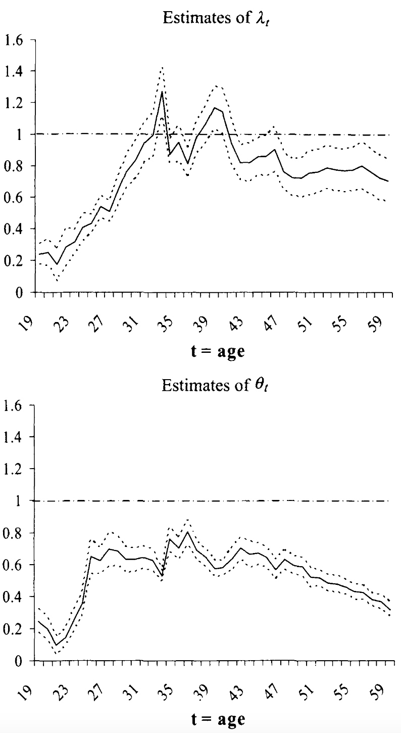
First, let’s consider latent endowment (for example, genetics). Let’s assume that income in each generation $t$, $y_{it}$, is determined by the endowment value of that generation $e_{it}$. The endowment process is an AR(1) process with persistence parameter $\lambda$. In this model,

$${\beta }_{-1}={\rho }^2\lambda {\beta }_{-2}={\rho }^2{\lambda }^2$$

It is now easy to see that ${\left({\beta }_{-1}\right)}^2-{\beta }_{-2}={\rho }^4{\lambda }^2-{\rho }^2{\lambda }^2=({\rho }^2-1){\rho }^2{\lambda }^2$. So, for $\rho \in [0,1]$ and $\lambda \in [0,1]$, the discrepancy is negative. We can also make this reasoning a little more refined and add human-capital accumulation in the picture. The result will be similar with a small adjustment for conversion of latent endowment to human capital. This framework allows us to reason about possible long-run effects of schooling reforms, for example. So, it can be that the reforms raise mobility within one generation by making schooling less dependent on family characteristics. However, if they do not affect the heritability of traits (for example, no changes to assortative mating), then these policies will not change long-run (multi-generational) mobility.

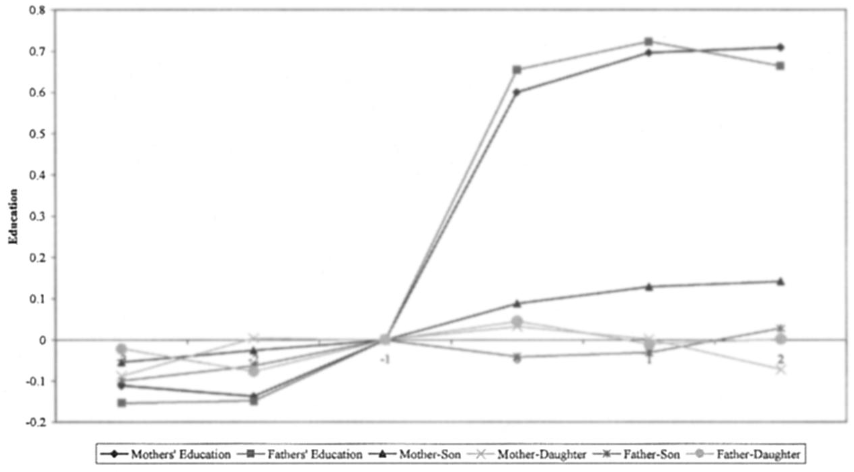
Second, children do not just inherit one endowment, but a whole host of them. Even if endowment is genetically transmitted, the genes determine numerous traits, which can enter the earnings process differently. So, suppose each generation has two endowments $e_{1it}$ and $e_{2it}$, each inherited with persistence ${\lambda }_1$ and ${\lambda }_2$ and entering the earnings process with coefficients ${\rho }_1$ and ${\rho }_2$. Then, the iterated regression fallacy parameter is negative as long as ${\lambda }_1\ne {\lambda }_2$. So, continuing with the genetic transmission example, $e_{1i}$ may be race (close to perfect heritability) and $e_{2it}$ cognitive intelligence (more malleable characteristic).

Third, as mentioned above, grand-parents and even more distant ancestors may have a direct impact on current generation, in addition to their indirect influence on parents. The expression for the discrepancy becomes massive and harder to interpret, but it also suggests that iterative parameter underestimates the long-run correlation.

Finally, Stuhler (2012) also describes a model with parental investments where $y_{i,t-1}$ enters into endowment generation process (for example, their investments into human capital) or directly in earnings process for $y_{it}$ (for example, parents’ networks may affect earnings of children besides the human capital channel). He shows that in the second case, the iterated regression fallacy can be biased in the opposite way if the direct impact of $y_{it-1}$ on $y_{it}$ is stronger than heritability of endowments.

Multigenerational mobility (Barone and Mocetti 2021)

Current individuals in Florence $\leftrightarrow$ ancestors in 1427 based on surnames

Source: Table 3 (Barone and Mocetti 2021)

There are also some creative papers that attempt to estimate intergenerational correlation over more than 3 generations. For example, Barone and Mocetti (2021) use surnames as the proxy for relationship between modern-day citizens in Florence and citizens in Medici time (XIV century). The measurement error in surname inheritance is likely to push the estimates towards zero. Despite that the authors find statistically significant estimates of intergenerational persistence. A 10% increase in ancestral income is associated with 4.5% higher earnings of modern-day descendants. Similarly, a 10% higher wealth associated with 1.8% higher wealth nowadays!

Multigenerational mobility (Collado, Ortuño-Ortín, and Stuhler 2023)

Horizontal approach: Grandparent-grandchild $\to$ cousin-cousin

• blood relationships: intergenerational processes

• in-law relationships: assortative processes

Swedish registry: “up to 141 distinct kinship moments”

Source: https://xkcd.com/2040

Alternatively, Collado, Ortuño-Ortín, and Stuhler (2023) are able to “capture” up to 141 generations by using the so-called horizontal chaining in the Swedish data. Using information on familial relationships (that directly may go up to 3-4 generations at most), they can link very distant cousins and cousins-in-law. Assuming that the processes are symmetrical for a pair of cousins, then their correlations can be expressed as a function of ${\beta }_{-k}$.

Multigenerational mobility (Collado, Ortuño-Ortín, and Stuhler 2023)

$$\begin{array}{rl}{y}_t& =\beta {\tilde{y}}_{t-1}+\gamma {\tilde{z}}_{t-1}+e_t+v_t+x_t+u_t\\ {\tilde{y}}_{t-1}& ={\alpha }_y{y}_{t-1}^m+(1-{\alpha }_y)y_{t-1}^f\\ {\tilde{z}}_{t-1}& ={\alpha }_z{z}_{t-1}^m+(1-{\alpha }_z)z_{t-1}^f\end{array}$$

$\beta$ and ${\alpha }_y$ measure direct transmission
$\gamma$ and ${\alpha }_z$ measure indirect transmission

$u_t$ is white noise (market luck)
$v_t$ is white noise in latent factor (endowment luck)
$x_t$ is shared sibling component
$e_t$ is latent sibling component

The framework used by Collado, Ortuño-Ortín, and Stuhler (2023) is described in the system of equations above. Outcome (for example, earnings) of current generation $y_t$ are determined in part by average outcome of parents, $y_{t-1}^m$ and $y_{t-1}^f$. Parents may have different functions and, therefore, enter differently in the earnings generation process. This is allowed by having ${\alpha }_y\ne 0.5$. Parents may also transmit other potentially unobserved characteristics, captured by $\widetilde{z_{t-1}}$. Again, this is a weighted average of unobserved characteristics of mother $z_{t-1}^m$ and father $z_{t-1}^f$.

Multigenerational mobility (Collado, Ortuño-Ortín, and Stuhler 2023)

	$\beta$	$\gamma$	${\alpha }_y$	${\alpha }_z$	${\sigma }_y^2$	${\sigma }_u^2$	${\sigma }_z^2$	${\sigma }_x^2$	${\sigma }_e^2$
Men	0.144	0.664	0.389	0.660	4.648	1.975	2.072	0.180	0.657
Women	0.129	0.566	0.018	0.775	4.465	2.333	1.559	0.244	0.712

Figure 1: Source: Table 4 (Collado, Ortuño-Ortín, and Stuhler 2023)

1. Indirect transmission dominates direct ($\beta <\gamma$)
2. Shared sibling component $x$ explains ~5%, $e$ ~ 15% of ${\sigma }_y^2$
3. Spousal correlation in latent factor $0.754={\rho }_{z^m{z}^f}>{\rho }_{y^m{y}^f}=0.489$ in observed characteristics

The main results of Collado, Ortuño-Ortín, and Stuhler (2023) are presented in the above table. First thing to note is that $\beta <\gamma$, both among men and women. This means that direct transmission of parents’ earnings to children’s earnings is dominated by the transmission of other characteristics that determine earnings of both generations. This can be genetic factors, non-cognitive factors, networks etc. Also, the latent endowments explain up to 45% of total variation in $y_t$.

It is also interesting that ${\alpha }_y<0.5$ meaning that father’s observed outcomes are more important in determining children’s earnings. But ${\alpha }_z>0.5$ meaning that mother’s latent characteristics are more important determinants of children’s outcomes.

When looking at variance components, the shared component between siblings (shared between all siblings to various degrees) accounts for 5% of total variance in $y_t$ and latent sibling component (only shared between same-gender siblings) - for 15%. This suggests that “most of the advantages that siblings share are not reflected in observables such as education or income”. Therefore, studies that use sibling correlations in these measures to capture shared family effects will also tend to understate intergenerational persistence.

Similarly, the authors find that spousal correlation in latent factors must be substantially higher than correlation in observed characteristics such as education or income to fit the patterns in the data.

Summary

• Vast literature on intergenerational mobility

  • Earlier works concentrated on measuring mobility precisely
  • Later works focus on determinants of mobility

• Improving access to education promotes mobility

  • The effect may spillover to children

• Geographic variation in mobility; largely causal

  • Lower segregation, inequality, better schools and social cohesion

• Genetic endowment and assortative mating important components

• Multigenerational mobility slower than predicted

References

Barone, Guglielmo, and Sauro Mocetti. 2021. “Intergenerational Mobility in the Very Long Run: Florence 1427–2011.” The Review of Economic Studies 88 (4): 1863–91. https://doi.org/10.1093/restud/rdaa075.

Becker, Gary S., and Nigel Tomes. 1979. “An Equilibrium Theory of the Distribution of Income and Intergenerational Mobility.” Journal of Political Economy 87 (6): 1153–89. https://www.jstor.org/stable/1833328.

———. 1986. “Human Capital and the Rise and Fall of Families.” Journal of Labor Economics 4 (3): S1–39. https://www.jstor.org/stable/2534952.

Black, Sandra E., and Paul J. Devereux. 2011. “Recent Developments in Intergenerational Mobility.” In Handbook of Labor Economics, 4:1487–1541. Elsevier. https://doi.org/10.1016/S0169-7218(11)02414-2.

Black, Sandra E., Paul J. Devereux, and Kjell G. Salvanes. 2005. “Why the Apple Doesn’t Fall Far: Understanding Intergenerational Transmission of Human Capital.” The American Economic Review 95 (1): 437–49. https://www.jstor.org/stable/4132690.

Chetty, Raj, and Nathaniel Hendren. 2018a. “The Impacts of Neighborhoods on Intergenerational Mobility I: Childhood Exposure Effects*.” The Quarterly Journal of Economics 133 (3): 1107–62. https://doi.org/10.1093/qje/qjy007.

———. 2018b. “The Impacts of Neighborhoods on Intergenerational Mobility II: County-Level Estimates*.” The Quarterly Journal of Economics 133 (3): 1163–1228. https://doi.org/10.1093/qje/qjy006.

Chetty, Raj, Nathaniel Hendren, Patrick Kline, and Emmanuel Saez. 2014. “Where Is the Land of Opportunity? The Geography of Intergenerational Mobility in the United States *.” The Quarterly Journal of Economics 129 (4): 1553–623. https://doi.org/10.1093/qje/qju022.

Colagrossi, Marco, Béatrice d’Hombres, and Sylke V Schnepf. 2020. “Like (Grand)parent, Like Child? Multigenerational Mobility Across the EU.” European Economic Review 130 (November): 103600. https://doi.org/10.1016/j.euroecorev.2020.103600.

Collado, M Dolores, Ignacio Ortuño-Ortín, and Jan Stuhler. 2023. “Estimating Intergenerational and Assortative Processes in Extended Family Data.” The Review of Economic Studies 90 (3): 1195–1227. https://doi.org/10.1093/restud/rdac060.

Corak, Miles. 2013. “Income Inequality, Equality of Opportunity, and Intergenerational Mobility.” Journal of Economic Perspectives 27 (3): 79–102. https://doi.org/10.1257/jep.27.3.79.

Fagereng, Andreas, Magne Mogstad, and Marte Rønning. 2021. “Why Do Wealthy Parents Have Wealthy Children?” Journal of Political Economy 129 (3): 703–56. https://doi.org/10.1086/712446.

Gelber, Alexander, and Adam Isen. 2013. “Children’s Schooling and Parents’ Behavior: Evidence from the Head Start Impact Study.” Journal of Public Economics 101 (May): 25–38. https://doi.org/10.1016/j.jpubeco.2013.02.005.

Goldin, Claudia, and Lawrence F. Katz. 2008. The Race Between Education and Technology. Harvard University Press. https://doi.org/10.2307/j.ctvjf9x5x.

Haider, Steven, and Gary Solon. 2006. “Life-Cycle Variation in the Association Between Current and Lifetime Earnings.” The American Economic Review 96 (4): 1308–20. https://www.jstor.org/stable/30034342.

Harden, K. Paige, and Philipp D. Koellinger. 2020. “Using Genetics for Social Science.” Nature Human Behaviour 4 (6): 567–76. https://doi.org/10.1038/s41562-020-0862-5.

Mazumder, Bhashkar. 2005. “Fortunate Sons: New Estimates of Intergenerational Mobility in the United States Using Social Security Earnings Data.” The Review of Economics and Statistics 87 (2): 235–55. https://www.jstor.org/stable/40042900.

Pekkarinen, Tuomas, Roope Uusitalo, and Sari Kerr. 2009. “School Tracking and Intergenerational Income Mobility: Evidence from the Finnish Comprehensive School Reform.” Journal of Public Economics 93 (7): 965–73. https://doi.org/10.1016/j.jpubeco.2009.04.006.

Pop-Eleches, Cristian, and Miguel Urquiola. 2013. “Going to a Better School: Effects and Behavioral Responses.” American Economic Review 103 (4): 1289–1324. https://doi.org/10.1257/aer.103.4.1289.

Rustichini, Aldo, William G. Iacono, James J. Lee, and Matt McGue. 2023. “Educational Attainment and Intergenerational Mobility: A Polygenic Score Analysis.” Journal of Political Economy 131 (10): 2724–79. https://doi.org/10.1086/724860.

Solon, Gary. 1992. “Intergenerational Income Mobility in the United States.” The American Economic Review 82 (3): 393–408. https://www.jstor.org/stable/2117312.

Stuhler, Jan. 2012. “Mobility Across Multiple Generations: The Iterated Regression Fallacy.” SSRN Electronic Journal. https://doi.org/10.2139/ssrn.2192768.

Suhonen, Tuomo, and Hannu Karhunen. 2019. “The Intergenerational Effects of Parental Higher Education: Evidence from Changes in University Accessibility.” Journal of Public Economics 176 (August): 195–217. https://doi.org/10.1016/j.jpubeco.2019.07.001.

Appendices

Head Start and absence of offsetting behaviour

Source: Table 2 (Gelber and Isen 2013)

Back

US Racial Dot Map

Chicago

Sacramento

Source: US Census Bureau

Back

White - blue

Black - green

Asian - red

Hispanic - yellow