6. Human Capital
KAT.TAL.322 Advanced Course in Labour Economics
Human capital
Labour heterogeneity is important for labour supply and demand.
Human capital includes education, training, health investments.
First references as early as Adam Smith; formalised by Becker in 1960s.
Stylised facts
Overview
Human capital is an investment
- benefit: gain in earnings
- cost: tuition, foregone earnings, psychological costs
Two main camps for source of gain in earnings:
- gain in productivity
- signalling
Earnings by education
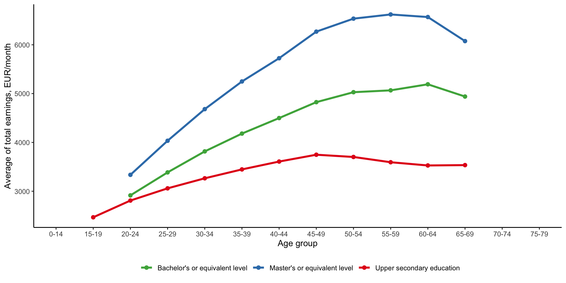
You might see this kind of figure a lot. It shows average monthly earnings of full-time workers by highest educational qualification across ages. There are two main observations we can get from this plot. Namely, that workers with higher education levels
- generally have higher level of earnings, and
- have faster earnings growth over time.
Both of these contribute to a substantial education premium in earnings over the lifecycle.
Human capital production function
Typically, univariate (years of education), it can be complex function of
- Innate skills (e.g., genetics)
- Parental investments (e.g., day care, time spent with children, tutors)
- Schooling/formal education
- Quantity (e.g., high school vs university)
- School quality (e.g., teacher quality, expenditure per student)
- Differences in curricula/fields (e.g., STEM vs arts)
- Peers (e.g., at school, at work)
- On-the-job training (e.g., general vs specific skills)
See Cunha and Heckman (2007) for a nice framework of pre-market production of skills
It’s worth mentioning that the term human capital is very vague. It is a set of all skills we have and acquire that help us produce some output. Even if we consider educational attainment as a measure of human capital, it can still mean a lot of things.
The most standard way is just to count years of education. It is the simplest and most universal variable available throughout the world. However, years of education may not capture the entirety of education (or human capital). For example, having 16 years of education with a bachelor degree can be valued differently from 16 years of same education but without the degree.
Besides the debate about productive and signalling value of education, the factors that create the education are numerous. Some of them are listed above. These factors can contribute differently to the overall output that we measure by years of education and/or qualifications. Therefore, change in overall education level can have different impact depending on which of these channels has generated the change.
In this lecture, we focus mainly on formal schooling and touch upon importance of innate skills and on-the-job training. For further discussion of determinants and consequences of education, you can check the references in the reading list.
Adult education
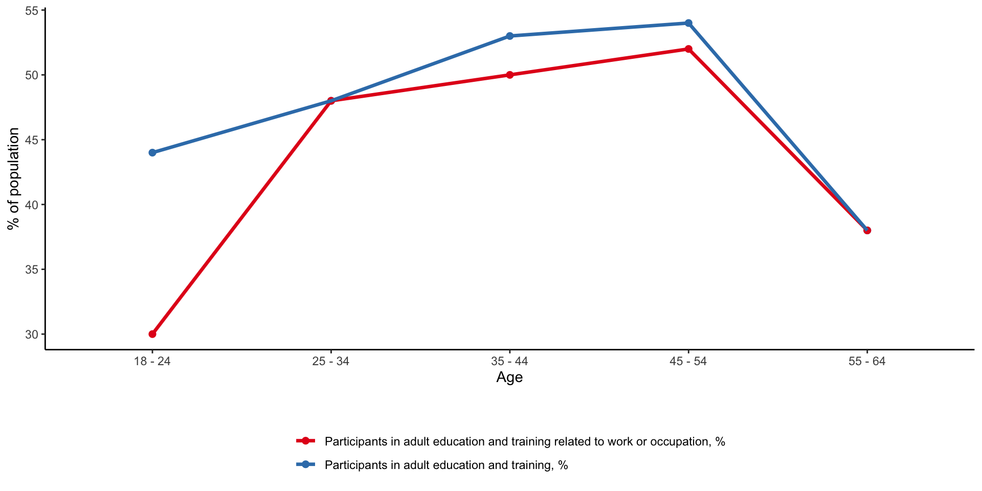
Another observation that we can explain in today’s lecture is participation in training after formal education has finished. The figure above plots share of population in a given age group that is participating in any form of adult education.
We can see that it tends to increase as people get older, but only up to a certain moment. Participation rate of pre-retirement age group - between 55-64 is much lower than participation rates of younger people.
We will see a model that aims to explain this lifecycle pattern in training.
Productive human capital investments
Basic model
Assume education choice \(S \in \{HS, C\}\)
Worker with \(S\) produces \(Y_S\) goods when employed by a firm
Perfect competition ensures that \(W_{HS} = Y_{HS}\) and \(W_C = Y_C\)
Assume cost of education given by function \(\eta(S)\)
Then choose college if marginal benefit outweighs marginal cost
\[ S = C \iff \color{#288393}{W_{C} - W_{HS}} \geq \color{#9a2515}{\eta(C) - \eta(HS)} \]
We begin with a static model with homogeneous workers and perfectly competitive employers.
A worker can decide how much education to acquire. For simplicity, we can make a binary decision between attending university or starting to work right after high school. We assume that level of education determines marginal productivity of each worker. In other words, in this model education enhances productivity. A worker with high-school diploma can produce \(Y_{HS}\) units of output, while one with university degree - \(Y_C\) units of output. Typically, we assume that \(Y_C > Y_{HS}\).
Under perfect competition we know that each worker is paid their marginal productivity. Therefore, worker with high-school diploma earns \(W_{HS} = Y_{HS}\) and one with university degree \(W_C = Y_C\).
If this were all, then everybody would be interested in getting university degree, which isn’t the case in real life. So, we must assume that education is costly. Note that even though this model is static, the cost function \(\eta(S)\) may include both direct costs of education as well as value of foregone earnings. The opportunity cost of foregone earnings is more apparent in a lifecycle model, which we will consider next.
A worker chooses to get university education if and only if her utility with univeristy education is at least as high her utility with only a high-school diploma. Here, we also implicitly assume linear risk-neutral utility function. Therefore, we can write down the decision rule using wages and cost of education directly. Therefore, the worker chooses \(C\) iff
\[ W_C - \eta_C \geq W_{HS} - \eta_{HS} \]
So, according to this model, people invest into education because it raises their productivity. It is worth noting that this investment decision will also be influenced by any possible market failures. In particular, it is one of the classical examples of positive externality. Raising education level of population may additionally benefit the society through better health, higher civic engagement, lower criminality, etc. All of these mean that social benefits of education may outweigh individual benefits (higher lifetime earnings). As a result, market equilibrium delivers lower education levels compared to equilibrium reached by the benevolent social planner. This is main reason why many countries around the world invest heavily into formal education.
Lifecycle model: simplified Ben-Porath (1967)
- Divide time between schooling/training \(\sigma(t)\) and working \(1 - \sigma(t)\)
- Law of motion of HC: \(\dot{h}(t) = \theta \sigma(t)h(t)\)
- Production function per worker: \(y(t) = Ah(t) \equiv w(t)\)
- Assume linear utility and no utility cost of \(\sigma(t)\)
\[ \Omega = \int_0^T \left(1 - \sigma(t)\right) Ah(t)e^{-rt} \text{d}t \qquad \text{s.t. HC law of motion} \]
Marginal return to HC effort \(\sigma(t)\) is
\(\frac{\partial \Omega}{\partial \sigma(t)} = -Ah(t)e^{-rt} + \int_0^T \left(1 - \sigma(z)\right) A\frac{\partial h(z)}{\partial \sigma(t)} e^{-rz} \text{d}z\)
\(\frac{\partial \Omega}{\partial \sigma(t)} = \color{#8e2f1f}{\underbrace{-Ah(t)e^{-rt}}_\text{foregone earnings}} + \color{#288393}{\underbrace{A\theta\int_t^T \left(1 - \sigma(z)\right) h(z) e^{-rz} \text{d}z}_\text{discounted future payoff}}\)
We have seen at the beginning that education decision may not be taken at a single point in time. Rather we continually make decisions about formal or informal education throughout our lives. We can study this dynamic decision-making using lifecycle model (Ben-Porath 1967).
Here, a worker has 1 unit of time at each \(t\). She needs to decide how much of this time to devote to training/education vs employment. Let \(\sigma(t)\) be the time spent in education at \(t\).
Education is still a productive activity. That is, the more time we spend on education, the higher is her human capital. To formalise this argument we write down the law of motion for human capital (recall that \(\dot{h}_t \equiv \frac{\partial h_t}{\partial t}\)) that you can see above. It essentially says that the speed with which we accrue human capital depends on
- individual heterogeneity \(\theta\)
- time spent in training \(\sigma(t)\)
- existing level of human capital \(h(t)\)
Thus, if someone is innately very good at learning, she will learn more and faster. If someone devotes a lot of time to education, she will learn more and faster. If someone already knows a lot, she will learn more and faster.
As before, the level of human capital determines marginal productivity of the worker \(y(t) = Ah(t)\). Here, \(A\) is a general technology of production that converts human capital into output.
Again, we assume perfect competition. Hence, equilibrium wages are equal to marginal productivity of worker \(y(t)\).
Finally, assume linear utility with no utility cost of \(\sigma(t)\). This means once again that consumption at \(t\) is equal to earnings at \(t\). The earnings at \(t\) is a product of \(w(t)\) and amount of time spent in employment at \(1 - \sigma(t)\).
This is true for every time \(t\). Hence, we can write down discounted lifetime utility given by \(\Omega\) above. The worker now needs to maximise \(\Omega\) with respect to \(\sigma(t)\) subject to the law of motion of human capital.
To solve this, take the first-order derivative of \(\Omega\)
\[ \frac{\partial \Omega}{\partial \sigma(t)} = -Ah(t)e^{-rt} + \int_0^T \left(1 - \sigma(z)\right) A\frac{\partial h(z)}{\partial \sigma(t)} e^{-rz} dz \]
To develop this further we need to know \(\frac{\partial h(t)}{\partial \sigma(t)}\). For this, we can turn to the law of motion of human capital.
\[ \frac{d h(t)}{dt} = \theta \sigma(t) h(t) \]
Divide both sides by \(h(t)\)
\[ \frac{d \ln h(t)}{dt} = \theta \sigma(t) \]
Now, let’s write the expression for the entire evolution of human capital since \(t=0\) until \(t\)
\[ \ln h(t) - \ln h(0) = \int_0^t \frac{\text{d}\ln h(z)}{\text{d}z}\text{d}z = \int_0^t \theta \sigma(z)\text{d}z \]
Exponentiate both sides and write down an expression for \(h(t)\)
\[ h(t) = h(0) \exp\left(\theta \int_0^t \sigma(z)\text{d}z\right) \]
Now, we are ready to take partial derivative of \(h(z)\) with respect to \(\sigma(t)\). First, notice that \(h(z)\) does not depend on future \(\sigma(t), ~ \forall t > z\). In these cases, the derivative is equal to zero. Otherwise, we need to differentiate the above expression.
\[\begin{align*} \frac{\partial h(z)}{\partial \sigma(t)} &= \frac{\partial}{\partial \sigma(t)} \left(h(0)\exp\left[\theta \int_0^z \sigma(s)ds\right]\right)\\ &= \underbrace{h(0)\exp\left[\theta \int_0^z \sigma(s)ds\right]}_{h(z)} \theta \frac{\partial}{\partial \sigma(t)} \left(\int_0^z \sigma(s)ds\right) = \\ &= h(z) \theta \underbrace{\frac{\partial}{\partial \sigma(t)} \left(\int_0^z \sigma(s)ds\right)}_\text{functional derivative} \end{align*}\]
The last term is a functional derivative of a function:
\[ \begin{align*} V[\sigma] &= \int \sigma(r) dr \Rightarrow \\ \int\frac{\delta V}{\delta \sigma(r)} \phi(r)dr &= \left[\frac{d}{d\varepsilon} \int \sigma(r) + \varepsilon \phi(r) dr\right]_{\varepsilon = 0} = \\ &= \int \phi(r) dr \Rightarrow \\ \frac{\delta V}{\delta \sigma(r)} = 1 \end{align*} \]
In our case, \(\phi(r) = 1, \forall r\). Therefore, the integral evaluates to 1, which leads us to conclude that functional derivative part is equal to 1. This means that
\[ \frac{\partial h(z)}{\partial \sigma(t)} = \theta h(z), \qquad \forall z \geq t \]
Plug this into the first-order derivative of \(\Omega\) with respect to \(\sigma(t)\) and you will get the second expression on the slide.
As highlighted above, the terms have economic meaning. The first term captures opportunity cost of foregone earnings. Whenever a worker devotes \(\sigma(t)\) to education, she loses the opportunity to earn wages in that time. The second term captures the expected benefit from higher earnings in the future due to higher productivity level.
Again, the optimal allocation of time is such that marginal cost of education (foregone earnings) is equal to marginal benefit of education.
Note that here we assumed that there is no other cost of education. If there is direct cost of education, the FOC above will be augmented to account for it.
Lifecycle model: simplified Ben-Porath (1967)
Optimal effort is zero at low efficiency \(\theta\) and high discount rate \(r\)
The change in marginal return over time is given by
\[ \frac{d}{dt}\left(\frac{\partial \Omega}{\partial \sigma(t)}\right) = A h(t) e^{-rt}(r - \theta) \]
If \(r > \theta\), then marginal return \(\uparrow\) over time, but is negative at \(T\):
\[ \frac{\partial \Omega}{\partial \sigma(T)} = -Ah(T)e^{-rT} < 0 \]
Hence, marginal return at every period is negative \(\Rightarrow \sigma^*(t) = 0 \quad \forall t\).
Take the derivative of \(\frac{\partial \Omega}{\partial \sigma(t)}\) with respect to \(t\) (using Leibniz rule) and substitute the law of motion of human capital
\[\begin{align*} \frac{\text{d}}{\text{d}t}\left(\frac{\partial \Omega}{\partial \sigma(t)}\right) &= -A\dot{h}_t e^{-rt} + rAh(t)e^{-rt} - A\theta \left(1 - \sigma(t)\right)h(t)e^{-rt} = \\ &= -A\theta\sigma(t)h(t) e^{-rt} + rAh(t)e^{-rt} - A\theta \left(1 - \sigma(t)\right)h(t)e^{-rt} = \\ &= Ah(t)e^{-rt}\left(r - \theta\right) \end{align*}\]
When \(r > \theta\), then all the terms in the above derivative are positive. Therefore, the marginal utility of time devoted to education is increasing over time.
Now, let’s look at the marginal utility of \(\sigma(t)\) again and evaluate it at \(t = T\). In the terminal period \(T\), there is no more discounted benefit of future payoffs (the integral evaluates to zero) and the marginal utility consists of solely the opportunity cost of foregone earnings. It’s easy to see that this part is negative (it’s a utility loss). Thus, the marginal utility at \(t= T\) is negative.
From this we deduce that marginal utility of \(\sigma(t)\) is even lower (more negative) at \(t <T\). In this case, the worker is better off not wasting any time on learning and devote all time to employment.
This result is saying that if an individual has very low efficiency in learning (low \(\theta\)) or she is very impatient (high \(r\)), then she has no interest in learning. That is, she either doesn’t benefit enough from extra training or she doesn’t care about future payoffs as much as she does about current utility.
Lifecycle model: simplified Ben-Porath (1967)
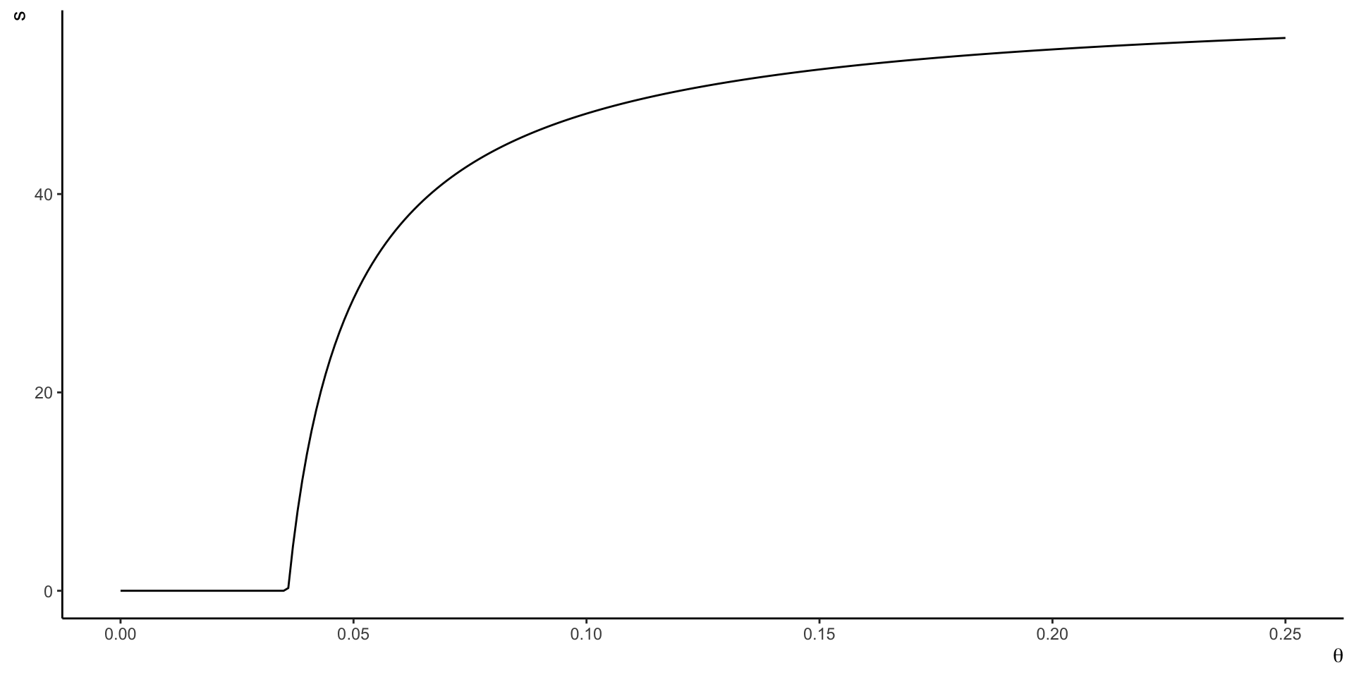
Optimal effort when efficiency \(\theta\) is high or discount rate \(r\) is low
Marginal return \(\downarrow\) over time \(\Rightarrow\) may exist \(t = s\) such that \(\frac{\partial \Omega}{\sigma(s)} = 0\)
- initial investment into education \(\sigma^*(t) = 1, \quad \forall t \leq s\)
- work rest of the time \(\sigma^*(t) = 0, \quad \forall t > s\)
- study longer if \(\theta\) higher
\[s = \begin{cases}T + \frac{1}{r}\ln\left(\frac{\theta - r}{\theta}\right) & \text{if } \theta \geq \frac{r}{1 - e^{-rT}} \\ 0 & \text{otherwise}\end{cases}\]
This is the opposite case of a worker with high efficiency \(\theta\) and/or more patience (lower \(r\)). From the derivative in the previous slide, we know that in this case marginal utility of \(\sigma(t)\) is decreasing over time. We also know that the marginal utility in the terminal period is negative. Therefore, we can conjecture that there may exist a point in time \(s\) such that marginal utility of \(\sigma(t)\) is exactly zero. If such time exists, then the worker is willing to devote all her time to education before \(s\) and has no interest in training after \(s\).
We can also write an explicit expression for \(s\) from the following equality
\[ Ah(s)e^{-rs} = A\theta \int_s^T \left(1 - \sigma(z)\right) h(z)e^{-rz}\text{d}z \]
From the previous derivations we have that
\[ h(t) = h(0) \exp\left(\theta \int_0^t \sigma(z)\text{d}z\right), \forall t \]
And we said that \(\sigma(t) = 1, \forall t \leq s\) and \(\sigma(t) = 0, \forall t > s\). Therefore,
\[ h(s) = h(0)e^{\theta s} \qquad\text{and}\qquad h(t) = h(s) ~ \forall t > s \]
Therefore, the equality of marginal utilities can be rewritten as
\[ Ah(s)e^{-rs} = A\theta h(s) \int_s^T e^{-rz}\text{d}z \]
After simplifying and rearranging we get
\[ e^{-rs} = \theta \frac{e^{-rs} - e^{-rT}}{r} \]
After further simplifications we can write
\[ s = T + \frac{1}{r}\ln\left(\frac{\theta - r}{\theta}\right) \]
You can also verify that \(\frac{\partial s}{\partial \theta} > 0\).
Lifecycle model: Ben-Porath (1967)
Allows for human-capital depreciation and on-the-job training
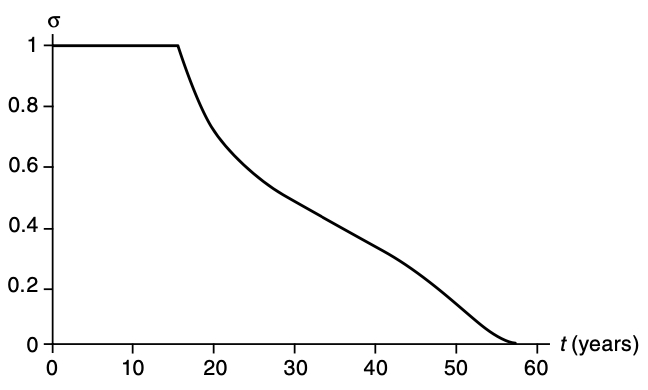
The full version of lifecycle model in Ben-Porath (1967) also allows for human capital depreciation over time. Therefore, workers have incentives to keep investing into learning after they fully enter labour market. However, similar forces are going to shape the optimal decisions here. Devoting time to learning means that the worker doesn’t earn as much. But acquiring more human capital helps to get higher earnings in the future. So, there is still going to be a point in time \(s\) where in all periods \(t \leq s\) individuals invest all their time on learning and after that they will start investing less. The closer the worker is to retirement, the lower are expected future benefits \(\Rightarrow\) invest less and less into education over time.
Signalling theory
Basic model
- Two types of productivity \(\theta_H\) and \(\theta_L\)
- Education \(e\) costs \(c_i = \frac{e}{\theta_i}\)
- Linear utility \(w - c_i, ~ \forall i \in \{H, L\}\)
Now, we consider the other camp of modelling investment into education. In this version, education is not a productive investment - it does not raise worker’s productivities directly. Instead, it is a tool that employers can use to learn about worker types.
The basic idea is that employers don’t have full information about workers. They don’t know actual worker productivities.
For simplicity, let’s start from the model where there are two types of workers \(\theta_L\) and \(\theta_H\) where \(\theta_L < \theta_H\) is actual productivity of the worker. So, \(\theta_L\) worker produces \(\theta_L\) units of output if employed.
Workers may choose to invest into education. It does not affect their productivities - those stay \(\theta_L\) or \(\theta_H\) fixed. But education is costly \(c_i\) and it is less costly for \(\theta_H\) workers \(c_H < c_L\). Workers’ utility is again linear and is equivalent to \(w_i - c_i\).
If employers did have full information, the we know that equilibrium under perfect competition is such that wages are equal to marginal productivities. Hence, \(w_H = \theta_H\) and \(w_L = \theta_L\).
Now, let’s imagine that employers announce that they pay \(w_H = \theta_H\) to anyone who acquires certain amount of education \(e\) and \(w_L = \theta_L\) otherwise. In this case, workers do have incentives to invest into education. The objective of an employer now is to set the required education level such that only \(\theta_H\) would want to get that level of education. This is called separating equlibrium.
Solution steps:
In a separating equilibrium, the types do not want to pretend to be of other types
\[\begin{cases} \theta_H - \frac{e_H}{\theta_H} \geq \theta_L - \frac{e_L}{\theta_H} \\ \theta_L - \frac{e_L}{\theta_L} \geq \theta_H - \frac{e_H}{\theta_L} \end{cases}\]
\(\Rightarrow \theta_L \left(\theta_H - \theta_L\right) \leq e_H - e_L \leq \theta_H \left(\theta_H - \theta_L\right)\)Given that costs \(c_L\) satisfies that above condition, we can find \(e_L^*\) that maximises individual payoff. This is easy, \(e_L^* = 0\) and her payoff is exactly \(\theta_L\).
Given the separation condition, the optimal education level of high type is \(e_H^* = \theta_L \left(\theta_H - \theta_L\right)\) and her payoff is \(\theta_H - \frac{\theta_L\left(\theta_H - \theta_L\right)}{\theta_H}\).
A few things to note:
Productive theory suggests that people under-educate themselves because of positive externalities. Signalling theory, however, says people overeducate themselves! Since education does nothing to productivity, it is only an annoying cost that people have to put up with. So, in the best-case scenario, nobody would get any education, but now they have to.
Notice that the equilibrium is equivalent to one achieved with full information. But workers have to pay extra cost of acquiring education. Thus, total welfare is lower.
Returns to education
J. Mincer (1958)
- \(E(S)\) earnings with \(S\) years of schooling
- Assume no direct cost of education
- Internal rate of return: \(r\) that equates costs and benefits
Present value of earnings \(P(S) = \int_S^T E(S) e^{-rt} dt = E(S) \frac{e^{-rS} - e^{-rT}}{r}\)
\[ P(S) = P(0) \Rightarrow \ln E(S) \approx \ln E(0) + rS \]
| Regression | \(R^2\) |
|---|---|
| \(\ln w = 7.58 + 0.070 S\) | 0.067 |
Linear utility, no direct cost, no heterogeneity => can estimate actual returns (net of costs = 0)
Otherwise, the estimates only show “revenue” side of story.
\[ \begin{align} P(0) &= E(0) \frac{1 - e^{-rT}}{r}\\ P(0) = P(S) &\Rightarrow E(0) \frac{1 - e^{-rT}}{r} = E(S) \frac{e^{-rS} - e^{-rT}}{r}\\ E(0)\left(1 - e^{-rT}\right) &= E(S)\left(e^{-rS} - e^{-rT}\right) \\ E(S) &= E(0) \frac{1 - e^{-rT}}{e^{-rS} - e^{-rT}} \\ E(S) &= E(0) e^{rS}\frac{1 - e^{-rT}}{1 - e^{-r(T - S)}} \\ \ln E(S) &= \ln E(0) + rS + \ln\left(\frac{1 - e^{-rT}}{1 - e^{-r(T - S)}}\right) \end{align} \]
J. A. Mincer (1974)
Accounting for experience
Building on Ben-Porath (1967)
- \(t(x)\) share of time dedicated to training at \(x\) experience and \(s\)
- HC law of motion: \(\dot{h}(s + x) = \rho_1 t(x)h(s + x), ~ \forall x \in [0, T - s]\)
\[\ln w(s + x) = \ln w(0) + \rho s + \rho_1 t(0) x - \rho_1\frac{t(0)}{2T} x^2\]
| Regression | \(R^2\) |
|---|---|
| \(\ln w = 6.20 + 0.107 S + 0.081 X - 0.0012 X^2\) | 0.285 |
Steps:
- Integrate HC law of motion: \(h(s + x) = h(s) e^{\rho_1\int_0^x t(v)dv}\)
- Assume again that \(w(t) = Ah(t)\); then
\[ \begin{align} w(s + x) &= Ah(s)e^{\rho_1 \int_0^x t(v)dv} = w(s) e^{\rho_1 \int_0^x t(v)dv}\\ \ln w(s + x) &= \ln w(s) + \rho_1\int_0^x t(v)dv \end{align} \] - Assume linear decay of training function: \(t(x) = t(0)\left(1 - \frac{x}{T}\right)\). Then
\[ \int_0^x t(0)\left(1 - \frac{v}{T}\right)dv = t(0)x - \frac{t(0)}{2T}x^2 \] - Plug in the above and \(\ln w(s) = \ln w(0) + \rho s\) into the expression in point 2
\[\ln w(s + x) = \ln w(0) + \rho s + \rho_1 t(0) x - \rho_1\frac{t(0)}{2T} x^2\]
Notes:
- Parameter \(\rho_1\) can be interepreted as the rate of return to on-the-job training
- Estimate of \(\rho \uparrow\)
- Signals that experience was an omitted variable and estimates on the previous slide likely suffer from omitted variable bias
- Experience and schooling are negatively correlated
OLS estimates of returns to schooling
Potential issues
Endogeneity of schooling and earnings
- Cognitive and noncognitive abilities (Heckman, Stixrud, and Urzua 2006)
Return to education is same regardless of duration of study
Does not take into account direct costs of education
Heterogeneity of returns (e.g., family background, schooling system)
Years of schooling vs qualifications
Productivity vs signalling interpretation
More on these in Card (1999)
Causal estimates of returns to schooling
Angrist and Krueger (1991)
Compulsory schooling laws: exogenous variation by quarter of birth
Instrumental variable approach
Local Average Treatment Effect (LATE)
\[ \begin{align} \ln W_{icq} &= \beta X_i + \rho E_i + \sum_c 1\{YOB_i = c\}\xi_c + \mu_i \\ E_{icq} &= \pi X_i + \sum_c 1\{YOB_i = c\}\delta_c + \sum_c\sum_q1\{YOB_i = c\} 1\{QOB_i = q\}\theta_{qc} + \epsilon_i \end{align} \]
Causal estimates of returns to schooling
Angrist and Krueger (1991)
IV estimates of returns to education \(\rho\)
| cohort30 | cohort40 | |
|---|---|---|
| r | 0.076 | 0.095 |
| (0.029) | (0.022) | |
| Weak IV F-stat | 1.6 | 3.2 |
Issues:
Instrument is weak (IV estimates are inflated)
Who are the compliers? Endogeneity? External validity?
Compliers represent only 0.46% of the population (extrapolation issue)
Compliers are also people that optimally choose min schooling
their baseline returns to schooling is likely to be low
but because of low base, an exogenous shift in years of schooling can overestimate marginal return to schooling among these people
Quarter of birth is a very weak instrument => estimates are inflated!
Trends within cohorts (may not have been fully accounted for by detrending and could reflect changes in the schooling system)
Endogenous choice of year and quarter of birth by parents
Causal estimates of returns to schooling
Some other IV approaches
| Instrument | Estimated \(\rho\) | |
|---|---|---|
| Card (1993) | Proximity to college | 0.132 (0.055) |
| Cameron and Taber (2004) | Proximity to college | 0.228 (0.109) |
| Cameron and Taber (2004) | Earnings in local labour market | 0.057 (0.115) |
| Kane and Rouse (1995) | College tuition fees | 0.116 (0.045) |
| Oreopoulos (2007) | Changes in compulsory schooling laws | 0.133 (0.0118) US 0.084 (0.0267) Canada 0.158 (0.0491) UK |
Causal estimates of returns to schooling
Twin studies
\[ \begin{align} \ln w_{ij} &= \alpha + \rho s_{ij} + A_j + \varepsilon_{ij}, ~\forall i \in \{1, 2\} \\ \Delta \ln w_j &= \rho \Delta s_j + \Delta \varepsilon_j \end{align} \]
| Estimated \(\rho\) | |
|---|---|
| Ashenfelter and Rouse (1998) | 0.088 (0.025) |
| Oreopoulos and Salvanes (2011) | 0.0476 (0.0026) |
Variation in schooling between twins \(\Delta s_j\) cannot be correlated with other variables that affect variation in earnings \(\Delta \ln w_j\)
- This is difficult to justify!
Causal estimates of returns to schooling
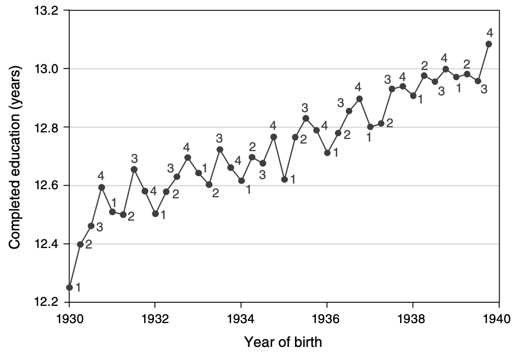
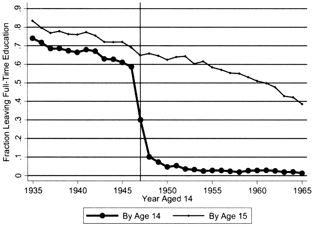
Regression discontinuity design: Oreopoulos (2006)
UK 1947: raised min school leaving age (ROSLA) from 14 to 15
Compare similar people just before and after policy change
Estimated \(\rho\) = 0.069 (0.040)
Second reform in 1972: min SLA \(\uparrow\) from 15 to 16
Small (or zero) return (Dickson and Smith 2011)
Potential questions:
- If returns are so high, why do they not stay up to age 15 to begin with?
Causal estimates of returns to schooling
Carneiro, Heckman, and Vytlacil (2011)
- Many papers estimate sizable returns to schooling
- Average dropout rate in OECD 17% in 2020
- Heterogeneity in returns to schooling
Role of individual characteristics? E.g., patience (Cadena and Keys 2015)
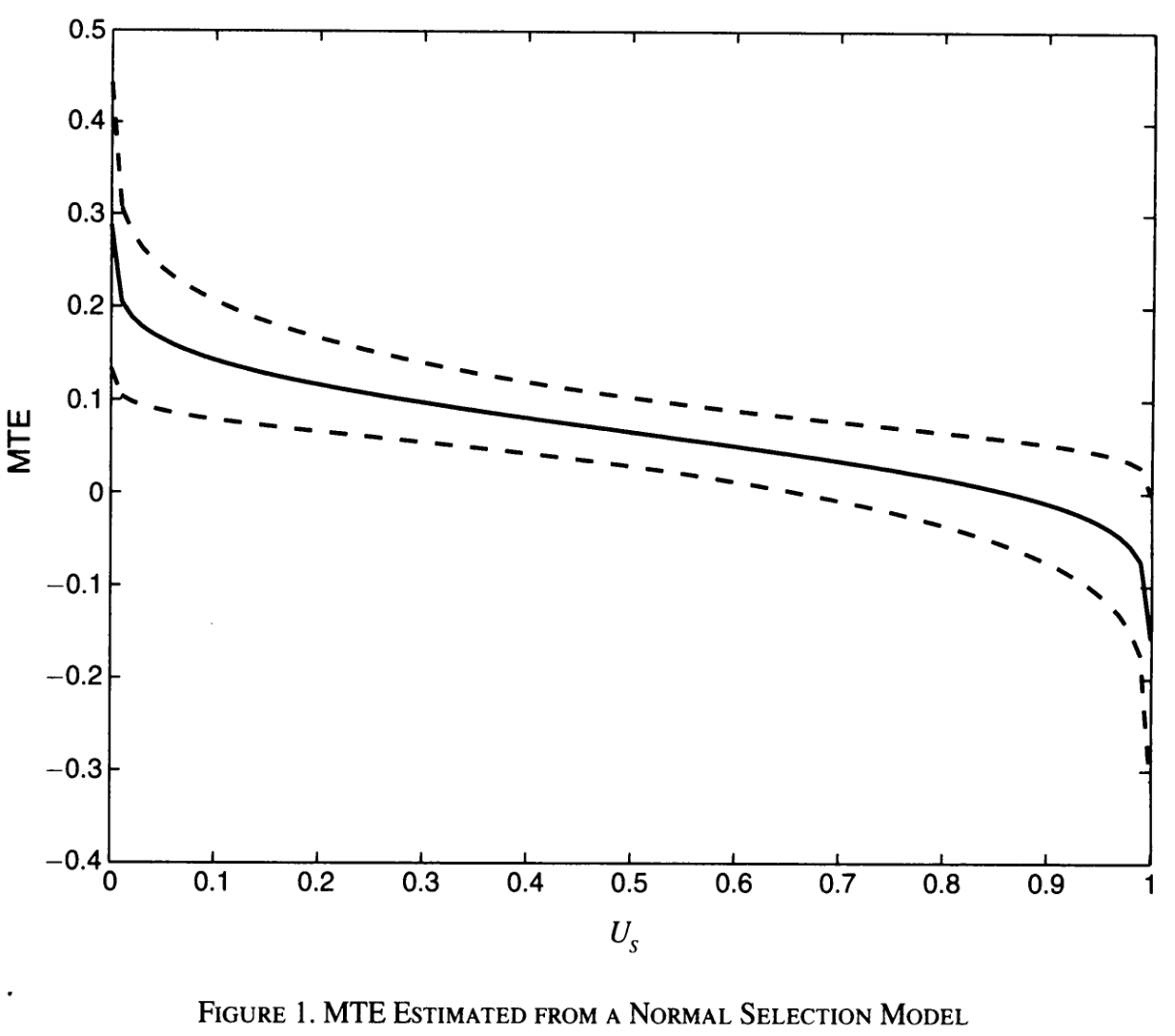
IV estimates = average of MTE, at best
Significant selection on gains:
dropouts already have very low returns (or negative)
those who stay have very high returns to education
Policy relevant effect thus depends on where along this curve the policy bites
Causal estimates of returns to schooling
Productivity or signalling?
Hard question to answer
Highlight that qualifications have both “productivity” as well as “signalling” parts
Summary
Education is a human capital investment
Models describing the investment decisions treat education as productivity enhancing and/or signalling device
Empirical estimates suggest sizable wage returns to a year of schooling
However, still a lot of debate about causality, heterogeneity and interpretation
Next lecture: Education Quality on 15 Sep
References
Angrist, Joshua D., and Alan B. Krueger. 1991. “Does Compulsory School Attendance Affect Schooling and Earnings?*.” The Quarterly Journal of Economics 106 (4): 979–1014. https://doi.org/10.2307/2937954.
Aryal, Gaurab, Manudeep Bhuller, and Fabian Lange. 2022. “Signaling and Employer Learning with Instruments.” American Economic Review 112 (5): 1669–1702. https://doi.org/10.1257/aer.20200146.
Ashenfelter, Orley, and Cecilia Rouse. 1998. “Income, Schooling, and Ability: Evidence from a New Sample of Identical Twins.” The Quarterly Journal of Economics 113 (1): 253–84. https://www.jstor.org/stable/2586991.
Ben-Porath, Yoram. 1967. “The Production of Human Capital and the Life Cycle of Earnings.” Journal of Political Economy 75 (4): 352–65. https://www.jstor.org/stable/1828596.
Cadena, Brian C., and Benjamin J. Keys. 2015. “Human Capital and the Lifetime Costs of Impatience.” American Economic Journal: Economic Policy 7 (3): 126–53. https://doi.org/10.1257/pol.20130081.
Cahuc, Pierre. 2004. Labor Economics. Cambridge (Mass.): MIT Press.
Cameron, Stephen V., and Christopher Taber. 2004. “Estimation of Educational Borrowing Constraints Using Returns to Schooling.” Journal of Political Economy 112 (1): 132–82. https://doi.org/10.1086/379937.
Card, David. 1993. “Using Geographic Variation in College Proximity to Estimate the Return to Schooling.” NBER Working Paper. Cambridge, MA. October 1993. https://doi.org/10.3386/w4483.
———. 1999. “The Causal Effect of Education on Earnings.” In Handbook of Labor Economics, 3:1801–63. Elsevier. https://doi.org/10.1016/S1573-4463(99)03011-4.
Carneiro, Pedro, James J. Heckman, and Edward J. Vytlacil. 2011. “Estimating Marginal Returns to Education.” The American Economic Review 101 (6): 2754–81. https://www.jstor.org/stable/23045657.
Chevalier, Arnaud, Colm Harmon, Ian Walker, and Yu Zhu. 2004. “Does Education Raise Productivity, or Just Reflect It?” The Economic Journal 114 (499): F499–517. https://www.jstor.org/stable/3590169.
Clark, Damon, and Paco Martorell. 2014. “The Signaling Value of a High School Diploma.” Journal of Political Economy 122 (2): 282–318. https://doi.org/10.1086/675238.
Cunha, Flavio, and James Heckman. 2007. “The Technology of Skill Formation.” American Economic Review 97 (2): 31–47. https://doi.org/10.1257/aer.97.2.31.
Dickson, Matt, and Sarah Smith. 2011. “What Determines the Return to Education: An Extra Year or a Hurdle Cleared?” Economics of Education Review, Special Issue: Economic Returns to Education, 30 (6): 1167–76. https://doi.org/10.1016/j.econedurev.2011.05.004.
Feng, Andy, and Georg Graetz. 2017. “A Question of Degree: The Effects of Degree Class on Labor Market Outcomes.” Economics of Education Review 61 (December): 140–61. https://doi.org/10.1016/j.econedurev.2017.07.003.
Heckman, James, Jora Stixrud, and Sergio Urzua. 2006. “The Effects of Cognitive and Noncognitive Abilities on Labor Market Outcomes and Social Behavior.” Journal of Labor Economics 24 (3): 411–82.
Kane, Thomas J., and Cecilia Elena Rouse. 1995. “Labor-Market Returns to Two- and Four-Year College.” The American Economic Review 85 (3): 600–614. https://www.jstor.org/stable/2118190.
Maurin, Eric, and Sandra McNally. 2008. “Vive La Révolution! Long‐Term Educational Returns of 1968 to the Angry Students.” Journal of Labor Economics 26 (1): 1–33. https://doi.org/10.1086/522071.
Mincer, Jacob. 1958. “Investment in Human Capital and Personal Income Distribution.” Journal of Political Economy 66 (4): 281–302. https://www.jstor.org/stable/1827422.
Mincer, Jacob A. 1974. Schooling, Experience, and Earnings. Book. National Bureau of Economic Research. https://www.nber.org/books-and-chapters/schooling-experience-and-earnings.
Oreopoulos, Philip. 2006. “Estimating Average and Local Average Treatment Effects of Education When Compulsory Schooling Laws Really Matter.” American Economic Review 96 (1): 152–75. https://doi.org/10.1257/000282806776157641.
———. 2007. “Do Dropouts Drop Out Too Soon? Wealth, Health and Happiness from Compulsory Schooling.” Journal of Public Economics 91 (11–12): 2213–29. https://doi.org/10.1016/j.jpubeco.2007.02.002.
Oreopoulos, Philip, and Kjell G Salvanes. 2011. “Priceless: The Nonpecuniary Benefits of Schooling.” Journal of Economic Perspectives 25 (1): 159–84. https://doi.org/10.1257/jep.25.1.159.