| year | N |
|---|---|
| 2004 | 5221 |
| 2005 | 5540 |
| All | 10761 |
Problem set to Lecture 2
Estimate labour supply elasticity
Data
This exercise uses EU-SILC public microdata from Finland that can be downloaded from https://ec.europa.eu/eurostat/web/microdata/public-microdata/statistics-on-income-and-living-conditions.
The documentation for the dataset (including variable descriptions) can be downloaded from https://circabc.europa.eu/ui/group/853b48e6-a00f-4d22-87db-c40bafd0161d/library/be52ec21-09db-4b2e-9998-97c27fb5db4d/details.
The dataset is a ZIP folder with yearly CSV files. You need household- and person-level datafiles for years 2004 and 2005:
- FI_2004h_EUSILC.csv
- FI_2004p_EUSILC.csv
- FI_2005h_EUSILC.csv
- FI_2005p_EUSILC.csv
Cleaning steps
Merge household- and person-level data separately for each year.
Household-level data contains variableHB030with unique household ID. Person-level data contains variablePB030with unique person ID. You can recover household ID in person-level data by removing the last 2 digits from person ID. Then, merge the household- and person-level data by year (HB010andPB010) and household ID.Select variables of interest.
PB010- Year of surveyHB030- Household IDPB030- Personal IDHH060- Current rent related to occupied dwellingHH070- Total housing costHS130- Lowest monthly income to make ends meetHY010- Total household gross incomePB140- Year of birthPB150- SexPL020- Actively looking for a jobPL040- Status in employmentPL060- Number of hours usually worked per week in main jobPY010G- Employee cash or near cash income
You may use other variables in the dataset. If you do, you should clearly specify which variable you are using and why.
For simplicity, keep only individuals
- who are or were employed (based on employment status variable),
- for whom looking for job indicator is missing (currently employed), and
- who work at least 25 hours in a week
- who are only observed once per year (there is one odd person ID which appears twice in 2005)
You should have 10 761 observations in total (see the tabulation below).
Prepare variables for the estimation
You can use variables for rent, housing cost or lowest monthly income to make ends meet to capture consumption value.
Make sure to clearly specify which variable you are using, how and why! That is, specify which variable from the dataset you use, any transformations you apply to it, where it enters in the regression equation and why you chose this variable.
Estimations
Estimate the cross-sectional elasticity in 2005 using regression Equation 1.
\[ \ln H_{it} = \alpha_w \ln w_{it} + \alpha_R \left(C_{it} - w_{it} H_{it}\right) + \theta X_{it} + v_{it} \tag{1}\]
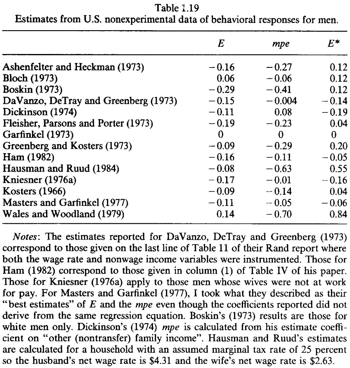
Report Marshallian wage elasticity, income effect and Hicksian wage elasticity given average value of wage and \(H_{it} = 40\).
Compare the estimates to those reported in Table 1.19 in Pencavel (1986)
Discuss possible issues with the estimates and suggest ways to mitigate these issues (either by using alternative estimation strategy or data source). Explain how the proposed solutions help improve the estimates. You do not need to implement these solutions.
Estimate the Frisch elasticity using regression Equation 2.
\[ \Delta \ln H_{it} = \rho + \alpha_w \Delta \ln w_{it} + \theta \Delta X_{it} + \Delta v_{it} \tag{2}\]
Report Frisch elasticity.
Discuss possible issues with the estimate and suggest ways to mitigate these issues. Explain how the proposed solutions help improve the estimates. You do not need to implement these solutions.
References
Pencavel, John. 1986. “Chapter 1 Labor Supply of Men: A Survey.” In Handbook of Labor Economics, 1:3–102. Elsevier. https://doi.org/10.1016/S1573-4463(86)01004-0.