9. Labour market discrimination

KAT.TAL.322 Advanced Course in Labour Economics

Same level of productivity, different outcomes based on nonproductive characteristics

• Employers may discriminate in hiring/firing decisions

• Co-workers may discriminate in collaboration activity

• Customers may discriminate in purchase decisions

Taste discrimination

Taste discrimination

First formalized by Becker (1957)

• There are two types of workers $A$ and $B$
• Perfect substitutes: $F(A+B)\Rightarrow F_A=F_B$

A firm decides how many workers to employ to maximise the utility

$$\underset{A,B}{max}PF(A+B)-w_{A}A-w_{B}B-dB$$

where $d\ge 0$ is the disutility employer gets from worker $B$

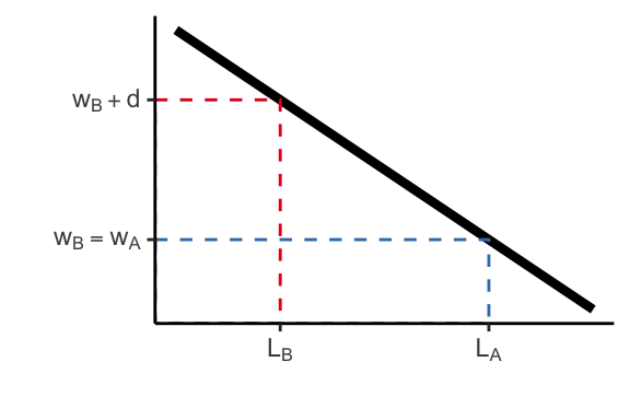
We start from a simple taste-based discrimination. Suppose we have two types of workers $A$ and $B$. These workers are otherwise identical and equally productive. The only thing that differs is their group identity. The identity itself does not enter into production function (unproductive characteristic).

The firm decides how many workers of each type to employ. In case where there is no discrimination $d=0$, it is easy to show that $w_A=w_B$ and labour demand $L_A=L_B$. But suppose that employer has some distaste for $B$ workers ($d>0$). This could be because the employer herself has distaste or because she expects the customers to discriminate against the firm based on $B$ employees. How does equilibrium look like in this case?

Taste discrimination

FOCs:

$$\begin{array}{rl}P{F}_A(A+B)& =w_A\\ P{F}_B(A+B)& =w_B+d\end{array}$$

Hire $B$ iff $w_B+d\le w_A$

Taste discrimination

Perfect competition and free entry

Non-discriminating firms $d=0$ enters the market

Pay competitive wages to both groups $w_A=w_B=P{F}_L(L)$

Therefore,

• discriminating firms hire $A$ workers at $w_A$
• non-discriminating firms hire everyone at $w_A=w_B=w$

Taste discrimination cannot persist under perfect competition

Taste discrimination

Imperfect competition

1. Monopsonistic employer

   Lower wages and lower employment of discriminated group

2. Market frictions (Black 1995)

   Job search costs:

   • Existence of employers with $d>0$ lowers reservation wage
   • Wages of discriminated workers at non-discriminating firms are also lower
   • Longer unemployment until meet non-discriminating firm

Statistical discrimination

Statistical discrimination

Overview

Key feature: unobservable productivity

• Suppose firms meets workers $A_i$ and $B_j$ such that $F_{Ai}=F_{Bi}$
• Firm doesn’t see $F_{Ai}$ or $F_{Bi}$, only group identities $A$ and $B$
• If firms believe that $\mathbb{E}(F_A)\ge \mathbb{E}(F_B)$, then $\uparrow w_A$ and $\uparrow L_A$

Statistical discrimination

• Two types of workers: high $h^{+}>0$ and low $h^{-}=0$

• Employers know the overall share of efficient workers $\pi (h^{+})\equiv \pi$

• Employers use costless test to infer worker types and hire if passed

  • $Pr(\text{pass}|h^{+})=1$
  • $Pr(\text{pass}|h^{-})=p$ where $p\in [0,1]$

• Average productivity of workers passing the test ($\equiv w$)

  $$w\equiv \mathbb{E}(h|\text{pass})=h^{+}\frac{\pi }{\pi +p(1-\pi )}$$

To demonstrate the concept of statistical discrimination, let’s actually abstract from group identities for now. We first demonstrate how wages and distribution of productivities are related. Once we see that, it is easier to analyse implications of different distributions between groups.

Let’s study a very simple environment with only two types of productivities - high ($h^{+}$) and low ($h^{-}$). Again, firms don’t see actual productivities $h^{+}$ or $h^{-}$. But they do know the probability distribution over them. In particular, the share of high-productivity workers is $\pi$ and of low-productivity workers - $1-\pi$.

Instead of paying average wages to everyone (and risk excluding the efficient workers from labour market altogether), firm decides to use a costless test to infer worker types. For example, think about tests developers need to pass to get an interview at Google, or trial periods in many firms. Let the test be such that high-productivity worker has no issue passing the test: $Pr(\text{pass}|h^{+})=1$. But also low-productivity workers may get lucky and pass the test with probability $p$: $Pr(\text{pass}|h^{-})=p\in [0,1]$.

The crucial information for the employer is the reliability of the test: how certain can the firm be that a worker that passed the test is actually high-productivity worker. Therefore, it is the conditional probability $Pr(h=h^{+}|\text{pass})$.

$$Pr(h=h^{+}|\text{pass})=\frac{Pr(h=h^{+}\text{ and pass})}{Pr\left(\text{pass}\right)}=\frac{\pi }{\pi +p(1-\pi )}$$

We assume that the firm hires everyone who passes the test. Therefore, average productivity of hired workers is

$$h^{+}Pr(h=h^{+}|\text{pass})+h^{-}(1-Pr(h=h^{+}|\text{pass}))=h^{-}+(h^{+}-h^{-})\frac{\pi }{\pi +p(1-\pi )}$$

Since we assume that firms are perfectly competitive, the wage the firm pays to its workers is equal to their average productivity. This wage is paid regardless of true type to anyone who passes the test.

Notice that the wage is increasing in $\pi$. Therefore, membership in groups with different $\pi$ will result in different wages. This is the essence of statistical discrimination. So, if worker $A$ and $B$ come from groups with different distributions of $h$ such that ${\pi }_A>{\pi }_B$, then also $w_A>w_B$ and $L_A>L_B$.

The wage is decreasing in the test error $p$. Suppose the test was perfect such that $p=0$. Then, only $h^{+}$ would be hired for wage $h^{+}$ and the rest would be hired for wage $h^{-}$. So, we could achieve the first-best equilibrium with full information. Conversely, if the test is completely useless $p=1$, then the firm learns nothing and has to pay uncondiational average of productivities to all its workers (pooling equilibrium).

Statistical discrimination

Self-fulfilling prophecies

Workers choose education to $\underset{e\in \{0,1\}}{max}U(w,e)=\underset{e}{max}w-e$

If $e=1\Rightarrow$ achieve productivity $h^{+}$, otherwise, $h^{-}$

$$\begin{array}{rl}{w}^{+}\equiv \mathbb{E}(h|\text{pass})& =h^{+}\frac{\pi }{\pi +p(1-\pi )}\\ \mathbb{E}(w|e=0)& =p{w}^{+}\end{array}$$

Optimal decision $e=1\iff w^{+}-1\ge \mathbb{E}(w|e=0)\Rightarrow p\le \pi \left[(h^{+}-1)(1-p)\right]$

The notion of statistical discrimination only tells that conditional on employers’ belief about the distribution, the discrimination between workers from different groups is optimal from profit-maximisation point of view. However, it does not explain where the belief comes from. If the underlying true distribution of productivities is, in fact, identical between group members, we would expect the employers’ belief to sooner or later converge to the true distribution. In this case, we should not observe statistical discrimination.

However, the beliefs held by employers can influence workers’ decisions and create self-fulfilling prophecies. Even if we start from an environment where workers in the two groups are identical to each other, the beliefs can encourage one group and discourage the other from investing into their human capital.

To see that, let’s consider the decision making of the workers. They have a simple linear utility of consumption with disutility from education. So, the workers must choose level of education $e$ that maximises her utility, balancing higher wages with utility cost of education. Let’s assume for simplicity that education decision is binary: she either pursues education $e=1$ or not $e=0$.

Given the firm’s optimal condition, the worker knows that if she achieves productivity $h^{+}$, she will get paid $w^{+}=h^{+}\frac{\pi }{\pi +p(1-\pi )}$. However, if she does not invest into education, she might still be paid same amount with probability $p$! She only chooses to invest into education if the extra payoff is sufficiently high to compensate for her utility loss from education.

It is easy to show that worker’s decision rule corresponds to the following equality

$$p\le \pi \left[(h^{+}-1)(1-p)\right]$$

Assuming that in full information, extra payoff is sufficient to compensate for utility loss ($h^{+}-1>0$), the worker only chooses to get education if

• test is sufficiently accurate $p\to 0$, or
• employer beliefs are sufficiently high $\pi \to 1$, or
• both.

In the equilibrium, the belief held by employers should be equal to share of workers pursuing education: $Pr\left(h^{+}\right)=\pi =Pr(e=1)$. Thus, this setup demonstrates that if employers (perhaps, irrationally) believe that ${\pi }_B<<{\pi }_A$, then workers in group $B$ have fewer incentives to actually invest into education and equilibrium settles such that, indeed, only share ${\pi }_B$ of workers in $B$ put effort to achieve $h^{+}$!

Statistical discrimination

Multliple equilibria and persistent inequalities

Source: Figure 5.7 (Cahuc 2004)

We can, in fact, plot worker utilities as a function of $\pi$ (for a given $p$). The red curve in the figure above shows utility of the worker without education, taking into account the optimal wages from firm decision. Similarly, the blue curve shows utility of the worker with education. The decision rule is simple: whenever $U(w,1)\ge U(w,0)$, worker gets education $e=1$. We can see that there is mid-point ${\pi }_0$ where the two utilities intersect. At this point, workers are indifferent between education or no education.

This means that there are three possible solutions in our simple model:

1. Firm believes there are no efficient workers $\Rightarrow$ no worker gets education
2. Firm believes all workers are efficient $\Rightarrow$ all workers get education
3. Firm believes share of efficient workers is ${\pi }_0\Rightarrow$ indifferent workers play mixed strategy with $Pr(e=1)={\pi }_0$.

All three of these cases satisfy optimality conditions of both workers and firms and the market clearing condition.

However, the last case with firms’ belief at ${\pi }_0$ is not a stable equilibrium. If, for some reason, the firm has a very slight error in its belief, i.e., ${\pi }_0\pm \epsilon$ for a very very small $\epsilon$, then the equilibrium quickly collapses to either one of the corner solutions. If error $\epsilon$ is positive, then the economy collapses to equilibrium where everyone gets education. If error $\epsilon$ is negative, it collapses to world where noone gets education.

It is now easy to see that if employers beliefs are ${\pi }_{0A}>{\pi }_{0B}$, then share of $B$ workers investing in education will be optimally lower in equilibrium.

In this sense, statistical discrimination can propagate economic inequalities and make them persistent.

Systemic discrimination

Systemic discrimination (Bohren, Hull, and Imas 2025)

Discrimination in one area has spillover effects on other areas

Let’s consider two programmers: male (M) and female (F)

So far, we considered discrimination somewhat isolated: discrimination on the part of employers at the hiring stage. However, discrimination can propagate throughout many different decisions that we have to make.

For example, we have shown that statistical discrimination by firms can discourage discriminated workers from pursuing higher education. Consider now the decision making problem of a university that needs to decide whether to admit a given student.

• One possibility could be that the admission officer cares about average earnings of graduates and bases admission decision on that. She sees that graduates from $B$ group still get lower wages than graduates from $A$ group. Then, she would optimally reduce share of $B$ students admitted to university.
• Another possibility is that the admission officer knows that students from groups $A$ and $B$ are equally capable, but employers hold wrong beliefs. She then decides to increase number of $B$ students admitted (hoping it will eventually push firms to correct their beliefs).

In both cases, discrimination in the labour market induces discrimination in university admission (either negative or positive). This is what’s called systemic discrimination in Bohren, Hull, and Imas (2025).

Systemic discrimination (Bohren, Hull, and Imas 2025)

Discrimination in one area has spillover effects on other areas

They submit codes $C_{0M}\equiv C_{0F}$ to open-source software

Systemic discrimination (Bohren, Hull, and Imas 2025)

Discrimination in one area has spillover effects on other areas

They receive performance ratings $P_M$ and $P_F$

Systemic discrimination (Bohren, Hull, and Imas 2025)

Discrimination in one area has spillover effects on other areas

Apply for jobs with signals $S_M=(P_M,R_M)$ and $S_F=(P_F,R_F)$

Systemic discrimination (Bohren, Hull, and Imas 2025)

Discrimination in one area has spillover effects on other areas

Employer’s hiring decision $A_M(M,S_M)$ and $A_F(F,S_F)$

The models we have seen so far help us think about direct discrimination in a given situation. For example, if there are two types of workers applying for a given vacancy, we want to know whether employer discriminate against one group holding all other characteristics constant! However, it has been recognised and showed in a number of papers that discriminated group must put in more effort to get same qualification as main group. For example, Hengel and Moon (2023) suggests that among papers published in top 5 economics journals, those authored by female economists are on average higher quality. This could suggest that publication threshold for female-authored papers is higher (or, alternatively, that female economists submit less often to top 5 journals). Another example documents that pull requests submitted by women on GitHub projects are less likely to be accepted (Terrell et al. 2017) and that female coders may receive lower performance rating for the same code (May, Wachs, and Hannák 2019).

The diagram above provides an illustration of the potential role of the systemic bias. Suppose we have two coders: male and female. Before they can start looking for jobs, they need to assemble their portfolio. They can do so by submitting their codes to open-source software. For example, Linux operating system is open-source and maintained by a group of enthusiastic coders. Since the software is open-source, individual coders do not receive wages or any other monetary compensation for submitting their codes to the repository. However, these codes can be evaluated, and the evaluation will become part of their portfolio. For example, you can imagine that each code is graded from 1 to 5 with 5 being highest grade. The coder then can approach an IT firm and present her CV and show the evaluations (grades) in her portfolio.

Now, imagine that our coders M and F submit exactly the same code to the open-source software (or, maybe not identical in content, but identical in quality). So, this is our way of saying that our coders have same initial coding ability (productivity). However, the evaluators happen to be biased against women for whatever reason. So, the female coder receives lower grade for the same quality of the code than male coder.

Next, both coders apply for jobs. They send their resumes of identical quality: it shows same qualifications, same experience. Employers might observe their grades for open-source contributions, in which, case they could use the lower evaluations to justify rejection of female candidate. Even if employers don’t see the grades directly, but have information that female coders usually get lower grades, they would still be less inclined to hire the female coder.

Typically, when we study discrimination, we want to hold all characteristics constant and only vary the variable of interest (in this case, gender). This illustration makes it clear that even when we exogenously equalize resumes and grades and find that no discrimination is taking place at the hiring stage, the discrimination still exists in the system and affects worker outcomes.

Decomposition (Bohren, Hull, and Imas 2025)

Direct discrimination

For a given signal $S$, $\delta (S)\equiv A(M,S)-A(F,S)\ne 0$

Total discrimination

Let $G(A|C_0,i)$ be distribution over all possible actions given identity $i$ and initial condition $C_0$.

$${\mathrm{\Delta }}^T(C_0)\equiv {\mathbb{E}}_G[A|C_0,M]-{\mathbb{E}}_G[A|C_0,F]\ne 0$$

Systemic discrimination

Let $\tilde{G}(A|C_0,i)$ be distribution over actions under original signal distribution but $A(-i,S)$

$${\mathrm{\Delta }}^S(C_0,M)\equiv {\mathbb{E}}_G[A|C_0,M]-{\mathbb{E}}_{\tilde{G}}[A,C_0,F]$$

$${\mathrm{\Delta }}^S(C_0,F)\equiv {\mathbb{E}}_{\tilde{G}}[A|C_0,M]-{\mathbb{E}}_G[A,C_0,F]$$

Decomposition

Let $\mathrm{\Sigma }(S|C_0,i)$ be distribution over all possible signals given identity $i$ and initial condition $C_0$

$${\mathrm{\Delta }}^T(C_0)={\mathbb{E}}_{\mathrm{\Sigma }}[\delta (S)|C_0,M]+{\mathrm{\Delta }}^S(C_0,F)$$

$${\mathrm{\Delta }}^T(C_0)={\mathbb{E}}_{\mathrm{\Sigma }}[\delta (S)|C_0,F]+{\mathrm{\Delta }}^S(C_0,M)$$

Direct discrimination can arise either due to preferences of decision makers (taste-based) or their beliefs about productivities/signals (statistical). Notice that we hold the signal that is available to the decision-maker constant. In our example, if programmers applied with same CVs $R_M=R_F$ and same performance ratings $P_M=P_F$, but we still observed difference in the hiring decision $A(M,S_M)\ne A(F,S_F)$, that would be evidence of direct discrimination by the employer.

Notice that direct discrimination can be identified at any stage in the process. For example, direct discrimination by the evaluators is $P(M,C_M)\ne P(F,C_F),\mathrm{\forall }{C}_M=C_F$.

Total discrimination accounts for discriminations that happen along the entire network given the individuals start with same initial condition $C_0$. So, it takes into account discrimination that could happen at the evaluation stage and at the hiring stage. Because the action set at each of these steps (nodes) may not be deterministic, we need to consider probability distributions. So, there is some probability distribution over performance evaluations that men and women get given the initial code $C_0$. This induces a probability distribution over signals that hiring manager sees and, consequently, probability distribution over actions that hiring manager can take for a given programmer that started with code $C_0$. These probability distributions will depend on the action rules at every preceding step, so can be expressed in terms of model parameters (see Section III in Bohren, Hull, and Imas 2025).

Systemic discrimination isolates all the preceding discrimination from the discrimination that might happen at the current step. We have our two programmers, who even though they submit same $C_0$, can receive different performance ratings $P_M,P_F$ and send different signals $S_M,S_F$ to employers. Letting all this to happen, suppose we had somehow convinced the employer that they are seeing $M$ instead of $F$ or vice versa. The signal would stay the same, but the employer is simply mistaken about the identity of the candidates they are seeing. So, from the employers perspective, they think they are considering $M$ with signal $S_F$ and $F$ with signal $S_M$ (instead of $M$ with $S_M$ and $F$ with $S_F$). Would we still see difference in outcomes between $M$ and $F$? If yes, we can conclude that there is discrimination in the preceding steps (signal generation). If not, then discrimination can only happen in the hiring stage.

Given all of this, we can also decompose total discrimination into average direct and systemic components. Thanks to this decomposition we can analyse relative importance of direct and systemic discriminations at different steps. Thus, we can analyse where along the path would reduction of discrimination be most effective.

Empirical results

Measuring discrimination

$\mathrm{\Delta }$ Wage by non-productive characteristics given same productivity.

Empirical challenges

• What constitutes a productive vs non-productive characteristic?
• Is $\mathrm{\Delta }$ wage attributable to discrimination alone or worker preferences?
• Does the discrimination arise from tastes or unobserved information?

Types of studies

• Observational
• Audit and correspondence studies
• Lab and field experiments
• Quasi-random variation

The idea behind discrimination of any kind is that outcomes of workers differ not because their true productivities differ, but because of some non-productive characteristic. However, it can be difficult to decide which characteristics are productive or not. For example, distribution of cognitive abilities are identical by gender, but distribution of physical strength can differ. Therefore, in jobs that mostly rely on cognitive functions gender can be considered unproductive characteristic, but in manual jobs - it can reflect differences in productivities.

It is also difficult to state to what extent differences between groups are attributed to discrimination or to differences in preferences between groups. For example, women often work in jobs that are closer and pay lower wages than men (Le Barbanchon, Rathelot, and Roulet 2020). Is this because discrimination happens that either women are only hired in lower-paying jobs, or discrimination happens where women can live, or because women have stronger preferences for commuting distances than for wages?

Finally, if we detect discrimination in the empirical work, can we tell if it arises because of tastes or statistical discrimination? This answer is crucial for policy implications of the findings. The set of policies that could effectively mitigate the discrimination will be very different depending on the source of discrimination.

Kitagawa-Oaxaca-Blinder¹ decomposition

Wages in two groups ($A$ and $B$) can be written

$$\begin{array}{rl}\ln w_A& ={\mathbf{x}}_A{\mathit{\beta }}_A+{\epsilon }_A,\mathbb{E}\left({\epsilon }_A\right)=0\\ \ln w_B& ={\mathbf{x}}_B{\mathit{\beta }}_B+{\epsilon }_B,\mathbb{E}\left({\epsilon }_B\right)=0\end{array}$$

Then, average wage differential

$$\mathrm{\Delta }\equiv \mathbb{E}(\ln w_A)-\mathbb{E}(\ln w_B)=[\mathbb{E}\left({\mathbf{x}}_A\right)-\mathbb{E}\left({\mathbf{x}}_B\right)]{\mathit{\beta }}_A+\mathbb{E}\left({\mathbf{x}}_B\right)({\mathit{\beta }}_A-{\mathit{\beta }}_B)$$

decomposed into explained and unexplained components.

First approach is to decompose observed differences in outcomes of two groups into explained and unexplained components. This decomposition is commonly used in many empirical works: it is easy to apply and interpret and does not require special data.

Let’s say we have data on wages, standard labour market characteristics (education, experience, occupation, etc.) and group identities (for example, male/female, native/immigrant, etc). We can estimate wage equations in two groups separately, relating their wages to the typical productive characteristics in $\mathbf{x}$.

Then, the difference in average wages can be written as

$$\mathrm{\Delta }\equiv \mathbb{E}(\ln w_A)-\mathbb{E}(\ln w_B)=\mathbb{E}\left({\mathbf{x}}_A\right){\mathit{\beta }}_A-\mathbb{E}\left({\mathbf{x}}_B\right){\mathit{\beta }}_B$$

Add and subtract $\mathbb{E}\left({\mathbf{x}}_B\right){\mathit{\beta }}_A$ to get

$$\mathrm{\Delta }=[\mathbb{E}\left({\mathbf{x}}_A\right)-\mathbb{E}\left({\mathbf{x}}_B\right)]{\mathit{\beta }}_A+\mathbb{E}\left({\mathbf{x}}_B\right)({\mathit{\beta }}_A-{\mathit{\beta }}_B)$$

The first term describes the explained differences. Basically, it is difference in composition of workers in the two groups by productive characteristics. For example, if all workers in $B$ have only 5 years of work experience, while all workers in $A$ have at least 30 years of experience, we can expect average wages in group $B$ to be correspondingly lower. So, if each year of experience in group $B$ was priced same way as in group $A$ (hence, using ${\beta }_A$), by how much we would expect their wages to be lower due to less experience?

The second term describes the unexplained differences. These differences arise because characteristics in ${\mathbf{x}}_B$ are priced in different way than in group $A$ (${\beta }_A-{\beta }_B$).

Kitagawa-Oaxaca-Blinder decomposition

Interpretation

• Common support: ${\mathbf{x}}_A$ and ${\mathbf{x}}_B$ contain same set of variables with similar value
• Conditional mean independence: $\mathbb{E}({\epsilon }_A|{\mathbf{x}}_A)=\mathbb{E}({\epsilon }_B|{\mathbf{x}}_B)=0$
• Invariance of conditional distributions: distribution of $w_A|{\mathbf{x}}_A$ remains unchanged if $B$ workers receive returns ${\mathit{\beta }}_A$

These are very strict assumptions, so the decomposition is a correlational (not causal) measure.

However, note that even if the second term is non-zero, it is not necessariliy an evidence of discrimination. Differences in ${\mathit{\beta }}_A$ and ${\mathit{\beta }}_B$ may arise for different reasons, including econometric issues.

First, the decomposition rely on ${\mathbf{x}}_A$ and ${\mathbf{x}}_B$ to have common support. It means both that

• they include same variables (i.e., same characteristics are relevant for productivities), and
• their distributions overlap.

The example we used about workers in $B$ only having 5 years of experience and in $A$ - 30 years, violates the common support assumption. We cannot identify ${\beta }_A$ for 5 years of experience or ${\beta }_B$ for 30 years of experience. In this case, the decomposition relies on extrapolation, which can be wildly inaccurate.

The conditional mean independence assumption is usual in many empirical studies. Basically, we want to the returns to observable skills captured by ${\mathit{\beta }}_A$ and ${\mathit{\beta }}_B$ to not be biased by unobservable characteristics. For example, if $A$ and $B$ are men and women, then returns to work experience may be biased for women if some confounding factor in ${\epsilon }_B$ affects both their wages and labour market participation. As you can see, without a plausibly exogenous variation induced by policy changes or controlled experiments, this assumption may be very difficult to satisfy.

The third assumption is there to exclude general equilibrium effects and self-selection into groups based on unobservables. For example, if women were paid the same way as men (${\mathit{\beta }}_B\equiv {\mathit{\beta }}_A$), the conditional distribution of men’s wages $w_A|{\mathbf{x}}_A$ would remain unchanged. This might not be the case if receiving ${\mathit{\beta }}_A$ would motivate significantly more women to participate in the labour market and, perhaps, pursue male-dominated occupations more often. You can imagine that, in this case, there will be general equilibrium effects on overall distribution of wages, so $w_A|{\mathbf{x}}_A$ is likely to change.

Kitagawa-Oaxaca-Blinder decomposition

Source: Table 8.5 (Cahuc 2004)

Nevertheless, the decomposition might still serve a useful descriptive measure that can be used to motivate a more thorough research question.

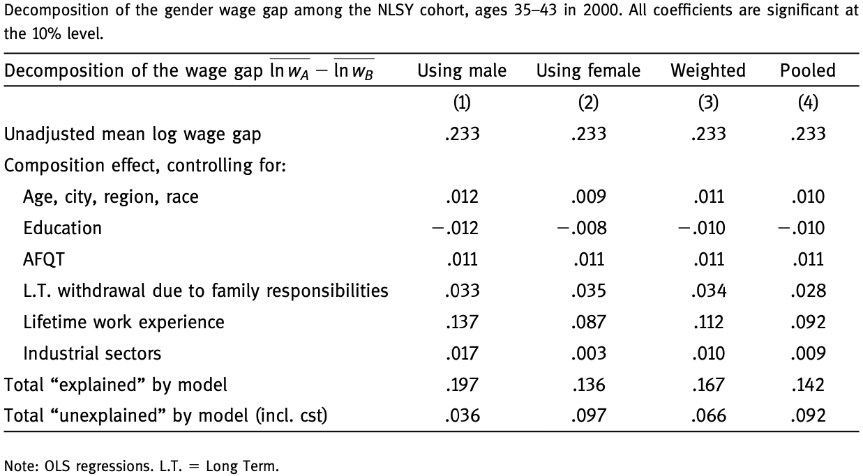
The table above shows the Kitagawa-Oaxaca-Blinder decomposition applied to gender gap in wages in the National Longitudinal Survey of Youth (NLSY) 1979 Cohort. The overall wage gap between men and women is about 23%.

Bulk of the total gender gap can be attributed to composition effect. About 60-70% of the composition effect is linked to differences in the overall work experience. This, in turn, accounts for about 50-60% of total wage gap. That is, men on average have more work experience, and, hence, earn higher wages.

The unexplained component accounts for only about 15% of the total wage gap. This could be due to other differences in labour markets of men and women and/or gender discrimination.

Notice that the choice of reference group can change the decomposition results considerably. When men are used as reference group, then 85% of the gender wage is attributed to explained component. Conversely, when women are used as reference group, then only 58% of the total wage gap is attributed to composition differences and 42% - to unexplained component. Can you explain why? Try to write out the decomposition formula with the opposite reference group.

Audit (correspondence) studies

• Send fictitious CVs nearly identical except in group membership
• Measure callback (interview invitations, offers) received
• RCT $\Rightarrow$ group differences can be interpreted as discrimination

Challenges

• CVs may not convey all relevant productive characteristics
• Cannot disentangle taste discrimination from statistical
• Harder to generalize

Audit or correspondence studies is basically a controlled experiment where a researcher can hold all observable characteristics equivalent and exogenously assign group membership to fictitious characters. For example, a typical setup is to generate a pool of CVs that are comparable in observable characteristics such as education, work experience and skills. Then, the researcher can randomly assign names that signal membership in a certain group. For example, male- and female-sounding names, or local- and foreign-sounding names.

Since group membership is assigned randomly any differences in outcomes between groups can be attributed to some form of discrimination.

Despite the advantages due to randomisation, correspondence studies have their own set of challenges.

• CVs may not convey all relevant productive characteristics

  For example, having a degree in computer sciences is a very coarse measure of skills; there’s still a lot of variation in programming skills among graduates with similar degrees. Alternatively, communication skills may be even more difficult to gauge from CVs alone without an in-person interview.

• Cannot disentangle taste discrimination from statistical

  All we get from the correspondence studies is that there are differences between groups, holding all else constant. But these differences may arise both because employers have certain beliefs about the groups the candidates belong to, or because employers simply prefer one group over another.

  A different type of experiment may be more useful for eliciting whether the discrimination happens because of preferences or beliefs. Given a pool of subjects (employers) that may have their beliefs about two different groups, we can randomly provide correct information to some of them. For example, suppose hiring managers believe that women prefer jobs that pay less, but have more flexibility. Let’s also say that we have results from a study that shows that this pattern is driven not by preferences, but by incomplete information, and that disclosing salaries earlier encourages more women to apply for better-paid jobs (Jalal, pre-published). If we give this information randomly to employers, do they adjust their behaviour (and maybe start disclosing salaries)? If so, then we could claim that the gaps existing before the experiment were driven by statistical discrimination.

• Harder to generalise

  Often, the outcomes that can be studied in the correspondence studies are just callback rates. Of course, if someone doesn’t get any callbacks, then it is unlikely they will get many interviews or offers. However, callback rates do not readily convert to interview invitations, job offers or conditions at next job (the variables that are more relevant for job-seekers and for policy-makers).

Bertrand and Mullainathan (2004)

Created templates for CVs of jobseekers in Boston and Chicago

• high and low quality types based on experience, skills, career profiles
• randomly assign distinctively White or African-American name
• track callback/email rates in race/sex/city/quality cell

	White names	African-American
College degree	0.720	0.720
	(0.450)	(0.450)
Years of experience	7.860	7.830
	(5.070)	(5.010)
Computer skills?	0.810	0.830
	(0.390)	(0.370)
Obs.	2 435	2 435

Source: Table 3 (Bertrand and Mullainathan 2004)

One of the seminal papers using correspondence study is Bertrand and Mullainathan (2004) where they investigate employer discrimination between White and African-American sounding names.

The authors generated a pool of fictitious CVs of two types: high- and low-skilled based on years and types of experience (volunteer experience, military experience), skills (computer skills, other special skills) and career profiles (including whether or not they had career breaks). They randomly assigned distinctively White or African-American sounding names to the CVs and sent them out to vacancies. The authors then tracked callback and email-back rates for each type of CVs.

The table above verifies that average quality of CVs between those assigned to White and African-American names are comparable. Therefore, any difference between these groups of CVs would be attributable to the names rather than differences in qualities.

Bertrand and Mullainathan (2004)

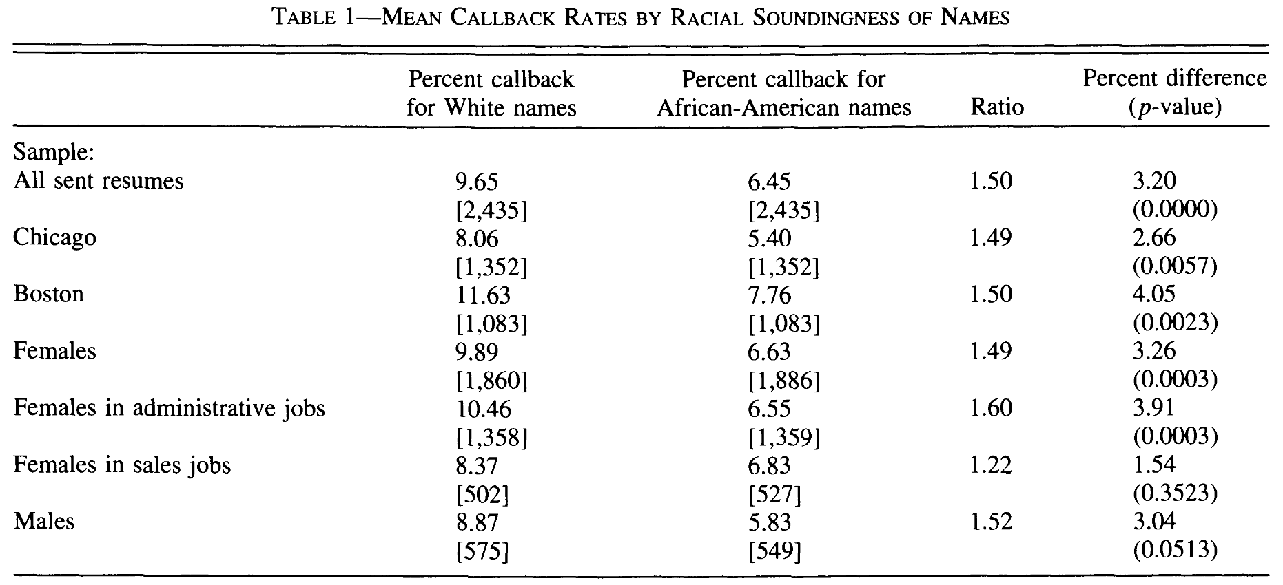
The table above shows the main results. We can see that CVs with White names received callback almost 10% of the time, while those with African-American names - 6.4% of the time. The difference is 3.2 percentage points and is statistically significant. The results are quite similar by geographic location and by gender. In addition to these results, Bertrand and Mullainathan (2004) also report that returns to quality of CV are lower for CVs with African-American names compared to White names. Higher-quality CVs with White names receive on average 3 pp more callbacks, while higher-quality CVs with African-American names only receive additional 0.5 pp more callbacks.

These results probably show the lower bound for discrimination.

• As mentioned earlier, callback rates are not equivalent to job offer rates. The gap may be larger at further stages of the candidate selection. However, the correspondence studies can only shed light on this very initial step of the process.
• The race is only communicated via name. Some employers might not pay much attention to names at such an early stage. Also, not all African-American citizens have distinctly African-American names. Both of these factors can contribute to even larger difference in outcomes at later stages.

Goldin and Rouse (2000)

Pre-1970s, musicians handpicked by the director

In 1970s-80s, auditions

• “open and routinized”
• blind (some stages)

Staggered adoption of screen: DiD method

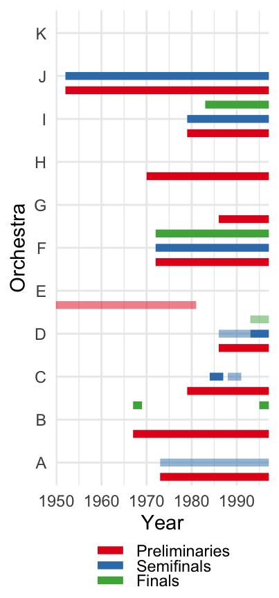
Goldin and Rouse (2000) exploit quasi-random variation introduced by a change in the audition process of musicians in orchestras. Before 1970s, the musicians were handpicked by the orchestra director personally. In 1970-80s, however, they re-organized the audition process considerably. Most notably, the auditions became more open and routinized. That is, there were now set periods of time when auctions were organised for major orchestras. This attracted more than 5x increase in the number of applications to the orchestras. To promote the selection by talent rather than connections or other characteristics, some orchestras also started implementing blind auditions (at least, at some stages of the selection).

These changes occurred at different points in time at different orchestras. Therefore, authors could study the implications of this policy change using difference-in-differences approach.

It is worth noting that since this is an actual policy change, the authors can study more relevant outcomes, such as job offer rates.

Goldin and Rouse (2000)

Results

	Preliminaries
	Without semifinals	With semifinals	Semifinals	Finals
Female x Blind	0.111	-0.025	-0.235	0.331
	(0.067)	(0.251)	(0.133)	(0.181)
Obs.	5 395	6 239	1 360	1 127
R2	0.775	0.697	0.794	0.878

Source: Table 6 (Goldin and Rouse 2000)

The table above shows the main results. The blind auditions improved the selection propensities of female candidates. The effects differ by the stage of the selection: significant and positive in preliminaries and finals, while strongly negative in the semifinals. The authors speculate that the negative effect at the semifinals could be related to special treatment of the semifinal round by the audition committee together with potential drive to explicitly advance women to finals. Therefore, committees in non-blind auditions would purposely advance female candidates to the finals, but they couldn’t do this positive discrimination when candidates are hidden behind screens.

Overall, however, the blind auditions significantly raised number of female musicians in orchestras. The effect comes both from higher probability of advancement and offer rates as well as higher number of female musicians applying to orchestras in the first place.

Mobius and Rosenblat (2006)

Lab experiment: taste discrimination based on beauty

Participants randomly assigned as workers (5) and employers (5).

1. Workers answer survey and solve simplest maze game

   Survey + practice time = digital CV

2. Confidence: predict # mazes solved in 15 min (private)

   $100A_j-40|C_j-A_j|$, where $A_j$ actual and $C_j$ predicted performance

We have mentioned that typical correspondence studies cannot differentiate between statistical and taste-based discrimination. To do this, we would need to hold beliefs of employers constant

In this lab experiment, Mobius and Rosenblat (2006) use graduate students who are randomly assigned to “worker” and “employer” roles.

1. In the very first step, workers complete a survey (gender, education, university, matriculation year, previous work experience, skills, hobbies) and solve simple maze game. These results form their digital CV.
2. In the second step, worker has to predict how many maze games she can solve in the next 15 minutes. This step measures the confidence level of the participants. She knows that her final payment will be penalized if she mispredicts her performence (either too high or too low). This ensures that participants are incentivised to predict truthfully. Workers’ estimates $C_j$ are kept confidential throughout the experiment. But the workers themselves may release this information at the next step of interviews. Therefore, having a measure of confidence can be useful in interpreting the results of the experiment.

Mobius and Rosenblat (2006)

3. Workers randomly matched to employers ($5\times 5$)

   B	CV only	(baseline)
   V	CV +	(visual)
   O	CV +	(oral)
   VO	CV + +	(visual and oral)
   FTF	CV + +	(face-to-face)

4. Employers set wages $w_{ij}$ = # mazes could solve in 15 min ${\mathrm{\Pi }}_i=4000-40\sum _{j=1}^5|w_{ij}-A_j|$

5. Workers complete 15 min “employment”: realised $A_j$

3. In the third step, “workers” are matched randomly to 5 “employers”. Each of the interactions is one of five types:
   • Baseline: see only CV
   • Visual: see CV with a photo
   • Oral: see CV and phone interview
   • Visual and oral: see CV with a photo and phone interview
   • Face-to-face: see CV with a photo and have in-person interview
4. Employers also need to predict # mazes each worker can solve in the 15-min period based on all the information they’ve received. The employers are also incentivised to provide true estimates of worker productivity: for every mispredicted maze, they receive 40 points less. Employers do the prediction step after they have met all 5 workers.

Highlight the logic after the next slide!

an employer with taste for beauty might want to sacrifice earnings by giving higher $w_{ij}$. But if she knows her wages won’t affect the worker, she has no incentive to do so.

Mobius and Rosenblat (2006)

6. Payoffs

   1. Firms receive ${\mathrm{\Pi }}_i$ as on previous slide

   2. Workers receive ${\mathrm{\Pi }}_j=100A_j-40|C_j-A_j|+\sum _{i=1}^5{W}_{ij}$ where $$W_{ij}=\{\begin{array}{ll}100w_{ij}& \text{with probability }80\mathrm{\%}\\ {\overline{w}}_j& \text{with probability }20\mathrm{\%}\end{array}$$

      Employers know if $W_{ij}=100w_{ij}$ before setting it!

5. After employers gave their estimates $w_{ij}$, workers complete their 15-min “employment”: they need to solve maze puzzles. This is used as actual realised productivity $A_j$ that is used when determining final payoffs.

6. All subjects receive their payoffs.

   The key part is that worker’s payoff depends on the “wages” set by employers. With 80% of chance they receive the exact wages a given employer set to them, and with 20% chance she earns average of all employers’ wages given to her.

Employers are told whether their $w_{ij}$ is used directly in worker’s payoff (instead of ${\overline{w}}_j$) before they give their estimates of $w_{ij}$ and after they have met all 5 workers. This is how the authors can capture taste-based discrimination: if employers have a taste for physically attractive workers, then they might be willing to provide higher over-estimated $w_{ij}$ in case they know the worker will directly benefit from it.

It is worth noting that the beliefs about productivities of workers are controlled in this experiment. The relevant information is obtained from the initial 5-minute practice run, which is disclosed to all employers.

Mobius and Rosenblat (2006)

Results

1. Beauty does not affect actual performance, but $\uparrow$ confidence

2. Beauty premia, but no taste-based discrimination

   	B	V	O	VO	FTF
   BEAUTY	0.017	0.131**	0.129**	0.124**	0.167**
   	(0.040)	(0.042)	(0.034)	(0.036)	(0.043)
   SETWAGE	-0.010	-0.072	0.098*	-0.046	0.033
   	(0.055)	(0.052)	(0.046)	(0.048)	(0.057)
   SETWAGE x BEAUTY	-0.058	-0.099+	0.005	-0.022	-0.044
   	(0.057)	(0.053)	(0.048)	(0.050)	(0.058)
   N	163	161	163	162	163

   Source: Table 4 (Mobius and Rosenblat 2006)

3. Beauty premium: 15-20% due to confidence, 40% - stereotype

In Table 3 (not shown here), Mobius and Rosenblat (2006) show that while beauty has no significant association with actual productivity of maze solving, it significantly raises confidence level of the participants.

The table above shows the results from the regression of $\ln W_{ij}$ on covariates of interest: beauty scale (ranked by high-school students outside of the experiment on scale from 1 to 5) and indicator for whether employers knew their wages enter worker’s payoff directly. We can see that in all interview types where there was either visual or oral “interaction” with workers, there is substantial beauty premium. Being more beautiful is associated with about 13% higher wages given by employers.

However, the interaction between beauty scale and $SETWAGE$ indicator is basically indistinguishable from zero. This suggests that employers in this experiment do not have taste for beauty.

If it is not taste-based discrimination for beauty, then what generates the beauty premia? The authors suggest that up to 20% of the beauty premium is due to confidence. We have mentioned earlier that beauty is positively associated with workers’ confidence. They could project this confidence in the oral and face-to-face interactions. And it could also explain why the beauty premium in FTF treatment arm is higher than the other visual or oral treatment groups. The residual beauty premia (after controlling for confidence levels), the authors attribute to visual or oral stereotypes. That is, for reasons other than confidence, people high on beauty scale may appear more able in front of the employers.

Rao (2019)

Field and lab experiments eliciting taste-based discrimination

$\mathrm{\Delta }$ policy in India: elite schools offer free places to poor students

Exploit staggered implementation using DiD

1. more charitable
2. changes fundamental notions of fairness and generosity
3. reduce discrimination (teammate choice in race)
   • high stakes: only 6% choose slower rich over faster poor student
   • low stakes: 33% discriminate against poor students
   • past exposure $\downarrow$ taste discrimination WTP by 12pp

Rao (2019) also studies taste-based discrimination, but using quasi-experimental variation induced by policy change in India. In particular, elite private schools at some point were required to offer free places to students from poor families. This induces a sharp discontinuity in the exposure of students from rich families to students from poor families.

Rao (2019) shows that cohorts with higher share of students from poor families become more charitable (do more volunteering activities).

He also measures their generosity in a lab setting using dictator game (player 1 has to decide how to split money between players 1 and 2, player 2 decides to accept or reject the split). He finds that students exposed to poor classmates are more likely to choose 50-50 split, irrespective of whether they are paired with poor or rich student. Therefore, he concludes that exposure to poor classmates changes the fundamental notions of fairness.

Finally, he uses a field experiment with the students in which they have to choose team-mates for a relay race. The results are that when stakes are high (winning prize equivalent to a month of pocket money), only 6% of students choose a slower rich teammate over a faster poor teammate. When stakes are low ($\times 10$ less than high prize), 33% of students choose slower rich teammates. However, being exposed to poor classmates previously reduces this discrimination by 12 pp. He estimates that rich students are willing to pay 2-days-worth of pocket money to avoid interacting with a poor student, but that past exposure to por classmates reduces the willingness to pay by nearly 13 times!

Doleac and Hansen (2020)

Quasi-random policy experiment measuring statistical discrimination

Ban-the-box (BTB) policy

• Banning prior criminal convictions box on job applications
• Hawaii in 1998 $⟶$ 34 states + DC in 2015

BTB “does nothing to address the average job readiness of ex-offenders”.

Therefore, statistical discrimination may $\uparrow$

Use DiD to measure effect of BTB on employment of minorities

Doleac and Hansen (2020) exploits a policy change in the US to elicit the strength of statistical discrimination in the labour market. In particular, she uses the so-called Ban-the-box (BTB) policy. Before the policy change job applicants were required to disclose their past criminal convictions on the application form. As the name suggests, the policy removed this box from the application forms.

The policy was intended at improving the re-employment prospects of past convicts. However, it did nothing in regards to maintaining or improving skills of ex-convicts. Therefore, the authors make a conjecture that removing this information could fuel statistical discrimination of non-criminal population.

Doleac and Hansen (2020)

	Full sample	BTB-adopting
White x BTB	-0.003	-0.005
	(0.006)	(0.008)
Black x BTB	-0.034**	-0.031**
	(0.015)	(0.014)
Hispanic x BTB	-0.023*	-0.020
	(0.013)	(0.015)
Obs.	503,419	231,933
Pre-BTB baseline
White	0.8219	0.8219
Black	0.677	0.677
Hispanic	0.7994	0.7994

Source: Table 4 (Doleac and Hansen 2020)

Indeed, the results show that employment of African-American and Hispanic workers reduces after the adoption of the BTB policy. The estimates are quite similar across different specifications, including restricting workers in control group to be from states that adopted the policy at some point (vs never-treated states used in the full sample).

To support the claim that this reduction in employment rates is driven by statistical discrimination, the authors show that

• the results are stronger in regions with higher share of Black and Hispanic workers;
• the results are stronger in periods of boom when employers can afford to exclude a large segment of labour market;
• the results are stronger among young male minority members, a demographic group with most ex-offenders with recent convictions.

Glover, Pallais, and Pariente (2017)

Capturing self-fulfilling prophecy of statistical discrimination

Quasi-random assignment of new cashiers to managers in French stores

Do minority cashiers perform worse with biased managers?

Measure manager bias using Implicit Association Test (IAT)

• 66% moderate to severe bias
• 20% slight bias

Outcomes: absences, time worked, scanning speed, time between customers

We have also seen a theoretical argument that statistical discrimination can trigger self-fulfilling prophecies. Glover, Pallais, and Pariente (2017) use quasi-random assignment of cashiers to managers in French stores. Their research question is whether ex-ante similar cashiers start performing worse with biased managers. The focus group are North or Sub-Saharan Africans starting cashier jobs (6 month contracts). They constitute up to 30% of all new cashiers.

Glover, Pallais, and Pariente (2017)

	Absences	Overtime (min)	Scan per min	Inter-customer time (sec)
Minority x Mngr bias	0.012***	-3.237*	-0.249**	1.360**
	(0.004)	(1.678)	(0.111)	(0.665)
Obs.	4,371	4,163	3,601	3,287
Dep var mean	0.0162	-0.068	18.53	28.7

Sources: Tables III and IV (Glover, Pallais, and Pariente 2017)

Indeed, the authors find that despite being comparable in pre-existing outcomes, exposure to biased manager makes cashiers less productive. It increases their absences, reduces their scanning speed and increases average amount of time between customers.

When digging deeper for explanations, the authors find that biased managers do not contribute to negative interactions between cashiers and managers. Rather there is less interaction, overall. So, for example, biased managers are less likely to chat with cashiers or ask them to do extra shifts. But this may come at a cost of hiring after the trial period, if these performance metrics are then used as the basis for the decision.

Another example of self-fulfilling prophecy: Carlana (2019) shows that ex-ante similar girls perform worse in math when exposed to biased teacher.

Bohren, Hull, and Imas (2025)

Role of gendered recommendation letters on hiring

• LLM: “female” and “male” recommendation letters
• Fictitious CVs with “male” and “female” names
• Survey 396 hiring managers

	Recommendation gender
CV name	CV	CV
	CV	CV

Finally, we also discussed systemic discrimination, i.e., discrimination in one setting provoking discrimination or contributing to different outcomes in another setting. The same authors Bohren, Hull, and Imas (2025) apply their proposed iterated correspondence study to gender gap in hiring and recommendation letters.

Job applications often require a recommendation letter from a previous employer or educational institution. It has been shown that there are significant differences between recommendation letters written for female and male candidates (Eberhardt, Facchini, and Rueda 2023). The letters written for women often use terms such as “nice” and “warm”, while those for men - “active” and “leader”.

How can we estimate the effect of gendered recommendation letters on hiring decisions and compare it to direct discrimination at the hiring stage? The authors approach this question using iterated correspondence study.

First, they generate a set of recommendation letters using LLMs. These letters display the typical features of recommendation letters written for men and women. They also generate a set of identical fictitious CVs where gender is signalled via distinctively female or male names.

Next, they surveyed 396 hiring managers that had previous experience in hiring for STEM jobs requiring recommendation letters. The managers were given a random set of two applicants, and they needed to report likelihood they’d advance the applicants to the next selection step and expected hourly wage.

The important feature of the experiment now is that there are four different types of application packages.

1. CV with a male name and male-language recommendation letter
2. CV with a female name and male-language recommendation letter
3. CV with a female name and female-language recommendation letter
4. CV with a male name and female-language recommendation letter

Thus,

• comparing the CVs 1 and 2 tells us about direct discrimination at the hiring stage under male action rule;
• comparing the CVs 2 and 3 tells us about systemic discrimination under female action rule;
• comparing the CVs 1 and 4 tells us about systemic discrimination under male action rule;
• comparing the CVs 1 and 3 tells us about total discrimination.

Bohren, Hull, and Imas (2025)

Hiring likelihood

Prospective wage

The results show that the extent of direct discrimination, both in hiring and wage setting, is much smaller than the extent of systemic discrimination stemming from gendered recommendation letters.

Systemic discrimination accounts for 95% of total discrimination in hiring probability and 136% of total discrimination in wages.

Summary

• Two main frameworks with different implications for labour markets

  • Taste-based discrimination
  • Statistical discrimination

• Systemic discrimination accumulating over time

• Simple decomposition to measure unexplained gap

• Vast experimental and quasi-experimental literature

Next lecture: Intergenerational mobility on 24 Sep

References

Becker, Gary S. 1957. The Economics of Discrimination. Economic Research Studies. Chicago, IL: University of Chicago Press. https://press.uchicago.edu/ucp/books/book/chicago/E/bo22415931.html.

Bertrand, Marianne, and Sendhil Mullainathan. 2004. “Are Emily and Greg More Employable Than Lakisha and Jamal? A Field Experiment on Labor Market Discrimination.” The American Economic Review 94 (4): 991–1013. https://www.jstor.org/stable/3592802.

Black, Dan A. 1995. “Discrimination in an Equilibrium Search Model.” Journal of Labor Economics 13 (2): 309–34. https://www.jstor.org/stable/2535106.

Bohren, J Aislinn, Peter Hull, and Alex Imas. 2025. “Systemic Discrimination: Theory and Measurement*.” The Quarterly Journal of Economics 140 (3): 1743–99. https://doi.org/10.1093/qje/qjaf022.

Cahuc, Pierre. 2004. Labor Economics. Cambridge (Mass.): MIT Press.

Carlana, Michela. 2019. “Implicit Stereotypes: Evidence from Teachers’ Gender Bias*.” The Quarterly Journal of Economics 134 (3): 1163–1224. https://doi.org/10.1093/qje/qjz008.

Doleac, Jennifer L., and Benjamin Hansen. 2020. “The Unintended Consequences of ‘Ban the Box’: Statistical Discrimination and Employment Outcomes When Criminal Histories Are Hidden.” Journal of Labor Economics 38 (2): 321–74. https://doi.org/10.1086/705880.

Eberhardt, Markus, Giovanni Facchini, and Valeria Rueda. 2023. “Gender Differences in Reference Letters: Evidence from the Economics Job Market.” The Economic Journal 133 (655): 2676–2708. https://doi.org/10.1093/ej/uead045.

Glover, Dylan, Amanda Pallais, and William Pariente. 2017. “Discrimination as a Self-Fulfilling Prophecy: Evidence from French Grocery Stores.” The Quarterly Journal of Economics 132 (3): 1219–60. https://www.jstor.org/stable/26372702.

Goldin, Claudia, and Cecilia Rouse. 2000. “Orchestrating Impartiality: The Impact of "Blind" Auditions on Female Musicians.” The American Economic Review 90 (4): 715–41. https://www.jstor.org/stable/117305.

Hengel, Erin, and Eunyoung Moon. 2023. “Gender and Equality at Top Economics Journals.” Working Paper. November 2023. https://erinhengel.github.io/Gender-Quality/quality.pdf.

Jalal, Amen. Pre-published. “Screening Women Out? Pay Transparency in Job Search.” https://amenjalal.com.

Le Barbanchon, Thomas, Roland Rathelot, and Alexandra Roulet. 2020. “Gender Differences in Job Search: Trading Off COMMUTE AGAINST WAGE*.” The Quarterly Journal of Economics 136 (1): 381–426. https://doi.org/10.1093/qje/qjaa033.

May, Anna, Johannes Wachs, and Anikó Hannák. 2019. “Gender Differences in Participation and Reward on Stack Overflow.” Empirical Software Engineering 24 (4): 1997–2019. https://doi.org/10.1007/s10664-019-09685-x.

Mobius, Markus M., and Tanya S. Rosenblat. 2006. “Why Beauty Matters.” The American Economic Review 96 (1): 222–35. https://www.jstor.org/stable/30034362.

Oaxaca, Ronald L., and Eva Sierminska. 2023. “Oaxaca-Blinder Meets Kitagawa: What Is the Link?” SSRN Electronic Journal. https://doi.org/10.2139/ssrn.4464602.

Rao, Gautam. 2019. “Familiarity Does Not Breed Contempt: Generosity, Discrimination, and Diversity in Delhi Schools.” American Economic Review 109 (3): 774–809. https://doi.org/10.1257/aer.20180044.

Terrell, Josh, Andrew Kofink, Justin Middleton, Clarissa Rainear, Emerson Murphy-Hill, Chris Parnin, and Jon Stallings. 2017. “Gender Differences and Bias in Open Source: Pull Request Acceptance of Women Versus Men.” PeerJ Computer Science 3 (May): e111. https://doi.org/10.7717/peerj-cs.111.

Footnotes

1. Formerly, Oaxaca-Blinder (Oaxaca and Sierminska 2023)