| Employed | Unemployed | Not working | |
|---|---|---|---|
| Sleep | 8.2 | 8.6 | 8.6 |
| Personal care and eating | 1.7 | 1.8 | 1.8 |
| Home production, shopping, care of others | 3.0 | 3.4 | 3.1 |
| Leisure, travel, sports and socialising | 5.3 | 8.2 | 7.6 |
| Work | 4.2 | 0.1 | 0.1 |
| Study | 0.1 | 0.1 | 1.1 |
| Unspecified | 0.1 | 0.1 | 0.2 |
4. Job Search
KAT.TAL.322 Advanced Course in Labour Economics
- No unemployment and perfect information in classical models
- Job search theory
- In classical model
- workers choose between working or not working (not participating in the labour market at all)
- if they chose not to work, they don’t spend time looking for a job
- Classical model also implicitly assumes perfect information
- workers know true characteristics of all the jobs in the market
- firms know true characteristics of all the workers in the market
- therefore, no need to “shop around” for a suitable job/worker
- Job search theory
- relaxes the assumption of perfect information, and
- studies the behaviour of workers looking for jobs
- is useful in analysis of aggregate unemployment rate and duration of unemployment spells among workers
- full equilibrium model with endogenous wage distribution is very useful for explaining wage inequality between otherwise identical workers
- this point is not explicitly discussed during the lectures
- if interested, do check out section 4 in chapter 5 of Cahuc, Carcillo, and Zylberberg (2014)!
Stylised facts
Time use by employment status
Source: Official Statistics of Finland (OSF) (2025)
- Substitution effect: return on job search \(<\) wage \(\Rightarrow \downarrow\) time searching
- Income effect: income unemployed \(<\) employed \(\Rightarrow \uparrow\) time searching
We will begin first by presenting some stylised facts that should clarify what kind of patterns the job search theories aim to explain. Note that this is often how economic models are presented in research papers. We develop models to explain a particular pattern of behaviour and outcomes we observe in the data. Therefore, presenting a set of stylised facts is often useful to describe these patterns and can then be later used to
- justify certain modelling decisions, and
- assess how well the model can explain these data patterns.
The main objective of job search models is to describe how people search for jobs. The table above shows average hours per day spent on various types of activities based on time use survey in Finland in 2009-2010. Unfortunately, the aggregate tables do not put job search activities into a separate category. However, by comparing the leisure hours between employed, unemployed (i.e., not working but looking for jobs) and non-employed (i.e., not working and not looking for jobs), it seems that job search is counted inside leisure group. The difference in leisure hours between unemployed and non-employed amounts to about 40 minutes. This is similar to 32 minutes spent on job search in the US reported in Table 5.1 of Cahuc, Carcillo, and Zylberberg (2014).
This might not seem like a lot of time. But this is an average number that can be “masking”
- variation over time, and
- variation between different groups of individuals.
Even employed workers will spend some time looking for jobs from time to time. Among unemployed workers, there are might be groups that search more intensively than others.
We will see that time people devote to searching for jobs is also an economic decision and depends on market conditions and social safety nets. The main trade-off we will consider is that in front of an unemployed individual that needs to decide whether to accept a job offer at some wage \(w\) or keep looking for a better job. And you can perhaps already see the opposing forces she has to take into account. If she accepts an offer, she starts receiving wages sooner. On the other hand, she is interested in finding best match for her to maximise income.
Job search is correlated with unemployment benefits
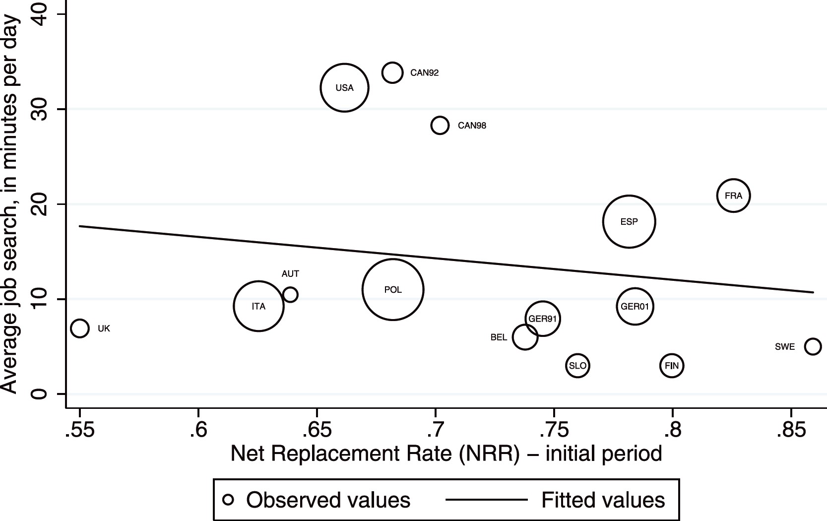
Since time spent looking for a job is an economic decision, it depends on market structure and social safety net. Thus, distribution of wages in the economy, availability of vacancies, competition for each vacancy all will affect her decision of when to stop looking for a job. Besides the market characteristics, unemployment benefits and re-employment public programs directly affect her decisions too. It is not surprising that one of the most-researched questions in this strand of literature looks at how unemployment benefits affect duration of job search and other outcomes of workers. Public funds is also a finite resource and we want to be able to spend this money effectively.
Past research shows that time spent looking for job is negatively correlated with access to financial resources. For example, Krueger and Mueller (2012) show that average time devoted to job search is lower in countries with higher unemployment benefits. In other words, in countries with low unemployment benefits, workers “try to find the next job as soon as possible”. In addition to formal unemployment benefits, many unemployed workers may rely on savings, income and assets of other family members.
You might be tempted to conclude from this graph that reducing unemployment benefits is the way to go. However, we will discuss briefly that the analysis might need to be a little more nuanced. First of all, when do people stop searching for jobs? It does not necessarily mean that they’ve stopped looking because they found a new job. Second, the graph above is silent about the quality of the next job. Can it be that higher benefits help workers find better-matched jobs?
Job search intensifies close to end of benefits

We will also see that job search intensity changes over time. This, too, can depend on markets, social safety nets and individual characteristics.
For example, the above graph is from Krueger and Mueller (2010) also look at average job search of unemployed workers over time in the US. The authors study job search behaviour around the time when government stops paying unemployment benefits after 26 weeks. You can see that many people intensify their job search in the last 6 weeks before the benefits run out. That too is a choice that can be rationalised in job search models.
Not all workers receive unemployment benefits
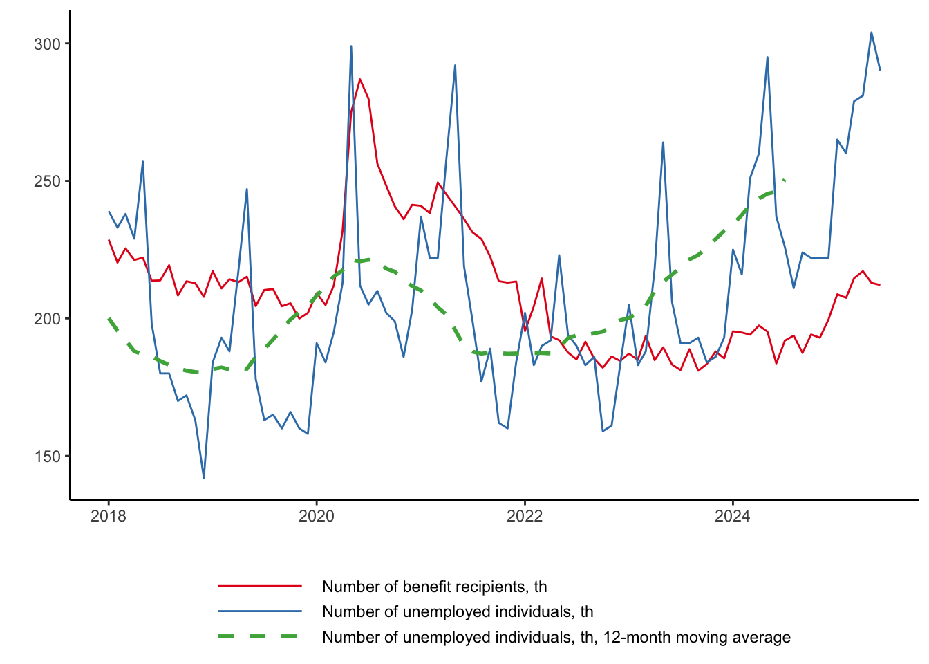
Understanding different forces shaping behaviour of workers that do and don’t receive unemployment benefits can be important in many countries. Even in Finland in recent years, there has been growth in number of unemployed individuals that do not receive any benefits.
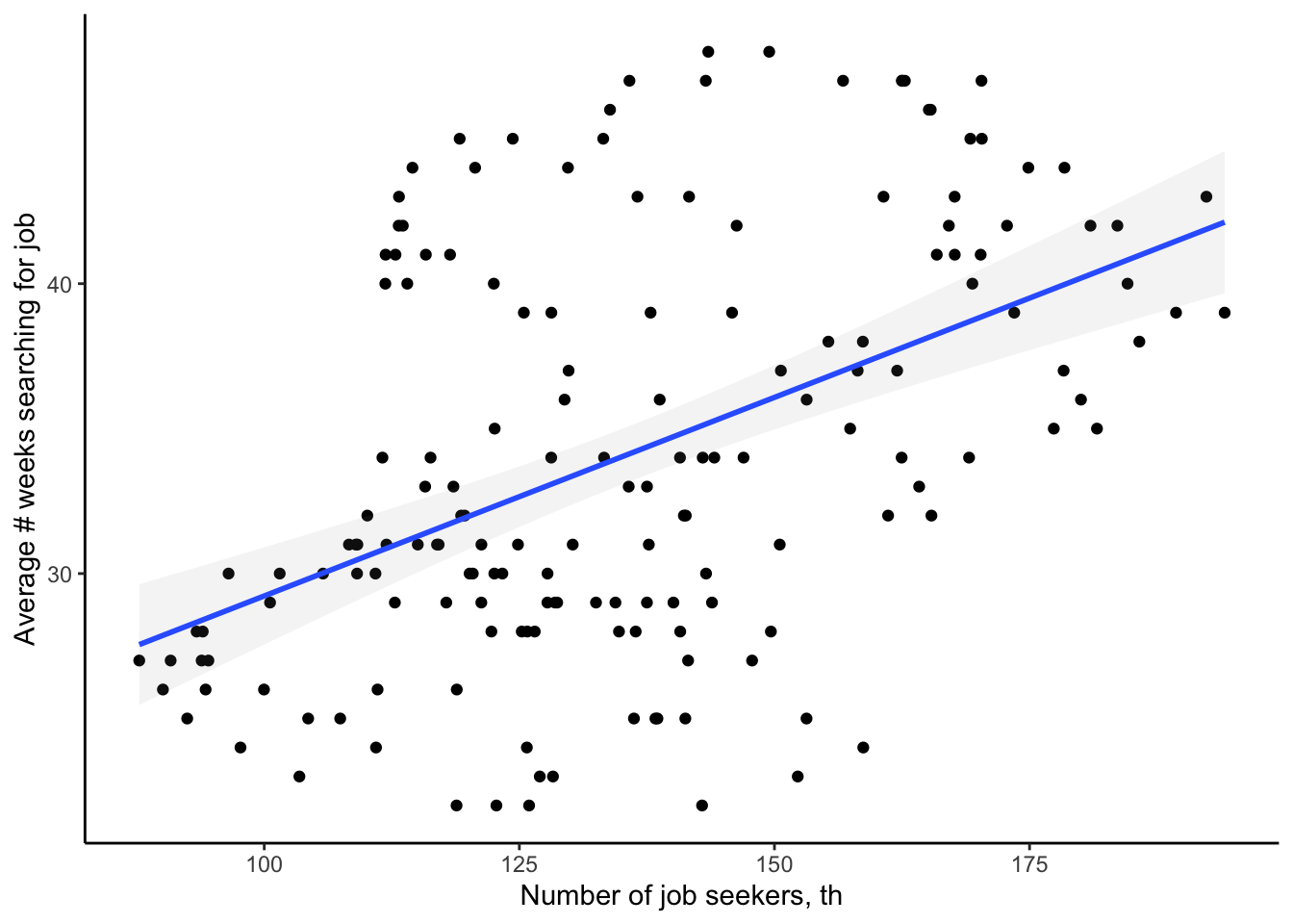
Job search longer when unemployment is high …
… and when there are more vacancies
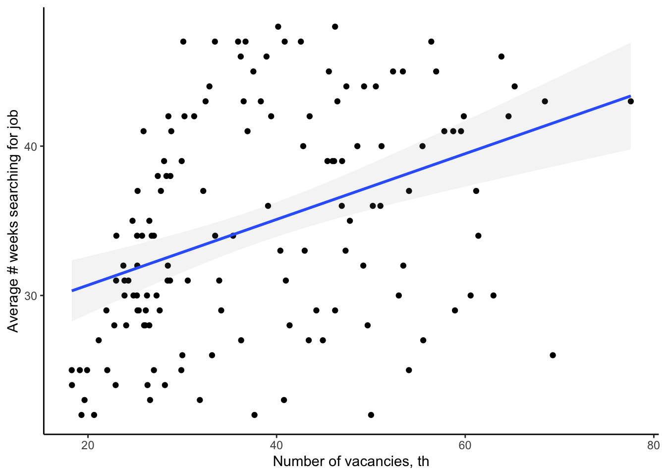
Though it is not a primary focus of basic job search models, but the search behaviour can also vary over the business cycle. The two graphs above illustrate that search behaviour depends not only on wages and benefits, but can also vary with number of unemployed individuals and number of available vacancies. You can think about what happens to these quantities in booms and recessions.
We will not cover it in today’s lecture, but a useful extension models a similar search behaviour on the firm side. These are usually called search and matching models, because workers and firms both decide on a match. These models can also help study the evolution of unemployment and vacancies over time.
Model
Basic job search model
- Workers do not know precise wage at each job, only CDF \(H(\cdot)\)
- Dynamic model with continuous time \(t\) (period is \(\text{d}t\))
- Key components
- Assume worker receives \(\leq 1\) job offer at wage \(w\) in period \(\text{d}t\)
- If she is employed with wage \(w\), assume her utility over \(\text{d}t\) is \(w~\text{d}t\)
- Exogenous job destruction at rate \(q~\text{d}t\)
- Discount future at rate \(\frac{1}{1 + r~\text{d}t}\)
- Let \(V_e\) and \(V_u\) be discounted utility of employment and unemployment
\[ V_e(w) = \frac{1}{1 + r~\text{d}t} \left(w~\text{d}t + \left(1 - q~\text{d}t\right)V_e(w) + q~\text{d}t~V_u\right) \]
In the basic model of labour supply there is no room for search. Workers know all relevant characteristics of all jobs available in the market and make their decisions based on that knowledge.
Therefore, modelling job search behaviour requires workers to not have full knowledge of job characteristics (wages, here). Instead, they only know the overall distribution of wages. For example, you may know that sales managers get on average around €8 000/month, nurses - €4 000/month, etc. But when you search for jobs, you may be offered lower or higher salaries than this average. In the model, worker learn wage \(w\) associated with a given job only after receiving an offer from that job.
Another critical component of search models is time dimension. You cannot study job search behaviour in a static model. We can specify time discreetly, \(t \in \{0, 1, \ldots \}\). However, it is customary to write down the search models in continuous time. It makes characterisation of an equilibrium a little easier. The period lengths \(\text{d}t\) can be arbitrarily small so that we could zoom-in to a decision where we need to make a decision about one job offer at a time. Instead, in discreet time it is possible that worker receives more than one job offer in a given period. Then, worker’s decision about each job might depend not only on that particular job, but also on set of other offers received in that period.
For simplicity, we assume that there is no leisure, non-wage income or savings, and that worker’s utility is a simple linear function of consumption, or equivalently, her earnings. The worker is also risk neutral.
For workers to find themselves in the position where they need to look for jobs, we must introduce job separations. The simplest way is to make it exogenous and constant at rate \(q~\text{d}t\). In extensions, you can also allow workers to make decisions about quitting jobs and/or firms to make decision about firing workers.
Since we have time component, we also need to introduce time discount factor. In continuous time, we can right it as \(\frac{1}{1 + r ~ \text{d}t}\), where \(r\) is the discount rate.
We can write down two value functions for this worker: value of accepting a job offer at wage \(w\) (\(V_e(w)\)) and value of rejecting the offer and continuing her search (\(V_u\)). The value of accepting the offer and becoming an employee with wage \(w\) consists of
- wage earnings received in a given period of time \(\text{d}t\)
- expected value of remaining at this job after \(\text{d}t\), which is just product of probability of not losing the job \(1 - q~\text{d}t\) and continuation value \(V_e(w)\)
- expected value in case she does lose a job, which a product of probability of losing the job \(q~\text{d}t\) and continuation value of unemployment \(V_u\).
Basic job search model and reservation wage
Optimal job search strategy
- If she receives no offer, she continues looking for a job
- If she receives an offer at wage \(w\), she accepts iff \(V_e(w) > V_u\)
Rewrite employee expected utility
\[ V_e(w) - V_u = \frac{w - r V_u}{r + q} \]
Since we assume \(V_u\) is constant, there is \(w^\star: V_e(w) > V_u ~~ \forall w > w^\star\)
It is easy to see that here \(w^\star = r V_u\)
\(w^\star\) is called reservation wage
Derivation steps:
Multiply both sides by \(1 + r~\text{d}t\)
\[ (1 + r~\text{d}t) V_e(w) = w~\text{d}t + (1 - q~\text{d}t)V_e(w) + q~\text{d}t~V_u \]
Add and subtract \(q~\text{d}t~V_e(w)\)
\[ (1 + r~\text{d}t) V_e(w) = w~\text{d}t + V_e(w) + q~\text{d}t\left(V_u - V_e(w)\right) \]
Simplify
\[ r~\text{d}t~V_e(w) = w~\text{d}t + q~\text{d}t\left(V_u - V_e(w)\right) \]
Divide by \(\text{d}t\)
\[ r V_e(w) = w + q\left(V_u - V_e(w)\right) \]
Add and subtract \(r V_u\) and rearrange
\[ V_e(w) - V_u = \frac{w - r V_u}{r + q} \]
We said that the worker will accept the job offer if \(V_e(w) \geq V_u\). Since \(V_u\) is constant in \(w\) and \(V_e(w)\) is increasing in \(w\), the two value functions cross only once. We usually call the wage at which the two values are equal the reservation wage. Hence, for any wage below \(w^\star\), \(V_e(w) < V_u\) and for any wage above \(w^\star\), \(V_e(w) \geq V_u\).
Now, we can easily see that at the reservation wage \(w^\star\)
\[ V_e(w) - V_u = \frac{w - r V_u}{r + q} = 0 \]
It follows from this that reservation wage of unemployed worker looking for job is \(w^\star = r V_u\).
This already helps us explain the positive relationship between duration of job search and level of unemployment benefits. It is reasonable to suspect that more generous benefits increase \(V_u\). The expression for reservation wages makes it clear that with higher \(V_u\), the reservation wage rises. This means that workers will search for longer time until they receive a wage offer above \(w^\star\).
Basic job search model and reservation wage
Expected utility \(V = \int_{-\infty}^{w^\star} V_u dH(w) + \int_{w^\star}^\infty V_e(w)dH(w)\)
Assume job offers arrive at an exogenous rate \(\lambda~\text{d}t\)
When unemployed, receive net income \(z \equiv b - c\)
- \(b\) is unemployment benefit, and
- \(c\) is total cost of job search (direct and indirect)
Can write \(V_u = \frac{1}{1 + r~\text{d}t}\left(z~\text{d}t + \lambda~\text{d}t V + (1 - \lambda~\text{d}t) V_u\right)\)
After simplifying and plugging in the expression for \(w^\star\), can show that \[ w^\star = z + \frac{\lambda}{r + q}\int_{w^\star}^\infty \left(w - w^\star\right) dH(w) \]
However, the relationship \(w^\star = rV_u\) is not very helpful because we don’t know \(V_u\). Before we can specify \(V_u\), we need to write down worker’s expected value ex-ante, i.e., before she gets any offer.
Even though she doesn’t yet get any offers, she knows they will come from the distribution \(H(w)\). She also knows that her decision rule is based on reservation wage. Therefore,
- for all possible wage offers below \(w^\star\), she assigns value \(V_u\), and
- for all possible wage offers above \(w^\star\), she assigns value \(V_e(w)\).
At this point, we also need to introduce the parameter that tells us how many job offers she receives. This is captured by \(\lambda ~\text{d}t\). In this basic model we also assume that \(\lambda\) is constant and exogenous. In reality, \(\lambda\) is likely endogenous and depends on
- state of the labour market and other aggregate costs of job search
- worker characteristics, such as age, education, occupation, etc.
- chosen effort of looking for job (active vs passive search)
Now, let’s think about \(V_u\). As in the case with employment value \(V_e(w)\), we can start from any benefits she receives or costs she incurs in current period. Let \(b\) capture the benefits and \(c\) capture cost of search. So, instead of earnings \(w\), she gets net benefit \(z \equiv b - c\). Cost of search \(c\) can include
- direct costs of job search (going to interviews, sending applications, etc)
- opportunity cost of time devoted to search.
In this period, she can also receive some offers at rate \(\lambda~\text{d}t\). In this case, she will be able to decide whether to accept or reject them. This value is captured by total expected value \(V\). She may also not receive any offers in that period, which happens at rate \(1 - \lambda ~\text{d}t\). In this case, she continues her search and receives value \(V_u\).
After following similar derivation steps as before, the expression for \(V_u\) can be written as
\[ r V_u = z + \lambda \int_{w^\star}^\infty \left(V_e(w) - V_u\right) dH(w) \]
After plugging in the expressions for \(V_e(w) - V_u\) and remembering that \(w^\star = r V_u\), it becomes
\[ w^\star = z + \frac{\lambda}{r + q}\int_{w^\star}^\infty \left(w - w^\star\right) dH(w) \]
Thus reservation wage depends on
- net income from unemployment \(z\)
- expected discounted value of accepted job offer (wage above \(w^\star\))
- offer arrival parameter \(\lambda\), and
- job separation parameter \(q\).
Basic job search model and unemployment duration
- Hazard rate, or exit rate from unemployment, depends on
- job offer arrival rate \(\lambda\)
- probability of offered wage being above \(w^\star \equiv 1 - H(w^\star)\)
- Hence, hazard rate is \(\lambda \left(1 - H(w^\star)\right)\)
- Average duration of unemployment is \(T_u = \frac{1}{\lambda\left(1 - H(w^\star)\right)}\)
The equation describing the reservation wage is useful for characterisation of worker behaviour. But it cannot be used in empirical estimations directly: reservation wages are unobserved!
We can, however, derive hazard rates (probability of stopping job search) and average duration of job search. These quantities are observed in real data and can be used in estimations.
So, first, let’s think about hazard rate. When does the worker exit unemployment in this model? When she receives a job offer AND she accepts it. The probability of offer arrival is \(\lambda\). The probability she accepts the job offer is same as the probability of job offer being above \(w^\star\), or \(1 - H(w^\star)\). Therefore, hazard rate is \(\lambda\left(1 - H(w^\star)\right)\).
It is also possible to show that average duration of unemployment is inversely proportional to hazard rate (see Cahuc, Carcillo, and Zylberberg (2014)). That gives us \(T_u = \frac{1}{\lambda\left(1 - H(w^\star)\right)}\).
Basic job search model and comparative statics
Using implicit differentiation, can show that reservation wage is
\[ \frac{\partial w^\star}{\partial z} > 0, \quad \frac{\partial w^\star}{\partial \lambda} > 0, \quad \frac{\partial w^\star}{\partial r} < 0, \quad \frac{\partial w^\star}{\partial q} < 0 \]
Therefore, average duration of unemployment is
- increasing in net income in unemployment: \(\frac{\partial T_u}{\partial z} > 0\)
- decreasing in interest rate: \(\frac{\partial T_u}{\partial r} < 0\)
- decreasing in job loss rate: \(\frac{\partial T_u}{\partial q} < 0\)
- ambiguous with respect to job offer arrival rate: \(\frac{\partial T_u}{\partial\lambda} \stackrel{?}{} 0\)
Now, we can derive a few comparative statics of interest. How do reservation wages \(w^\star\) and average duration of unemployment \(T_u\) vary with respect to the model parameters?
We can find the necessary partial derivatives using implicit function differentation. Derivation steps:
Rewrite the last expression for \(w^\star\) as
\[ \Omega(\cdot) = w^\star - z - \frac{\lambda}{r + q}\int_{w^\star}^\infty \left(w - w^\star\right) dH(w) = 0 \]
Compute partial derivatives of \(\Omega(\cdot)\) with respect to variables of interest and plug into implicit differentiation formula
Thus, the basic model is telling us that
with more generous unemployment benefits, jobseekers stay unemployed longer
Even though the prediction is unambiguous, magnitude of this relationship is unknown. Moreover, some empirical studies show that increasing benefits can actually shorten unemployment duration among workers who received no benefits at all.
unemployment duration increases when interest rates are high
When interest rate is high, an individual cares less about the future and more about current utility. Her reservation wage is lower and, consequently, spends less time looking for a job.
people spend less time looking for a job when chance of losing the job is higher
Remember that in this model once the worker accepts the offer, she sticks to the job until exogenous event forces her to quit. Therefore, when \(q\) is higher and she accepted an offer barely higher than \(w^\star\), she knows that very quickly she’ll be looking for job again and will have a chance to get an offer at even higher wage. Conversely, when \(q\) is low, once she accepts the offer, she is stuck at the job for longer period.
unemployment duration may increase or decrease with job offer arrival rate depending on how strongly the reservation wage reacts to \(\lambda\)
If reservation wage does not react to \(\lambda\), i.e., \(\frac{\partial w^\star}{\partial \lambda} = 0\), then average duration of unemployment decreases with \(\lambda\). This makes sense: the more offers a worker receives, the sooner she will get one above her reservation wage. However, worker can also become picky about jobs (her reservation wage \(\uparrow\)) and spend even more time looking for best job.
Job search with benefit eligibility
Two types of unemployed: eligible (\(V_u\)) and non-eligible (\(V_n\))
- Non-eligible earns income \(z_n < z\)
- All workers who have worked at least once are eligible
Expected utility of accepting offer same: \(r V_e(w) = w + q\left(V_u - V_e(w)\right)\)
Reservation wage of non-eligible worker satisfies \(V_e(w^\star_n) = V_n\)
Expected utility of non-eligible unemployed worker is \(r V_n = z_n + \lambda \int_{w^\star_n}^\infty \left(V_e(w) - V_n\right) dH(w)\)
Using all of the above, we can write \(w^\star_n\) as
\[ r w^\star_n = (r + q) z_n \color{#8e2f1f}{ - q w^\star} + \lambda \int_{w^\star_n}^\infty \left(w - w^\star_n\right)\text{d}H(w) \]
Can show that \(\frac{\partial w^\star_n}{\partial z} < 0\) and \(\frac{\partial T_n}{\partial z} < 0\)
In many countries, not all unemployed workers are eligible for unemployment benefits. Even in Finland you need to qualify for certain conditions to be eligible for some of the benefits. There are three types of unemployment benefits
- labour market subsidy: no work requirement, but assess need for the subsidy
- basic unemployment allowance: \(\geq\) 12 months of work history and salary above certain level; fixed amount irrespective of prior wages
- earnings-related unemployment allowance: \(\geq\) 12 months of work history and salary above certain level; benefit amount depends on prior wages
In this extension of the model, we will quickly study how does worker behaviour changes when she may not be eligible for benefits. We will see at the end that increasing unemployment benefits will have different impact on the behaviour of eligible and non-eligible workers. Therefore, policies that aim to reduce benefit sizes are going to incentivise some workers and discourage others.
Model
Consider a non-eligible unemployed worker that received a wage offer \(w\). Her expected utility of accepting the job offer is same as that of unemployed person and consists of instantenous utility \(w\) and weighted drop in utility if she looses this job \(q\left(V_u - V_e(w)\right)\). Since she has already been employed, even after losing this job, she will be unemployed worker eligible for benefits \(\Rightarrow\) the expected utility depends on \(V_u\) (and not on \(V_n\)).
The expression for expected utility of non-eligible unemployed worker is derived as follows. Notice that while she is unemployed, she earns \(z_n\). With probability \(\lambda\) she receives an offer that she can either reject or accept and with probability \(1 - \lambda\) she remains a non-eligible unemployed worker. The optimal strategy is still the same: accept offers above reservation wage and reject the rest. The only difference is that now she has her own reservation wage \(w^\star_n\), which may be different than \(w^\star\) of eligible unemployed worker. Therefore, the expression for her discounted expected value can be written as
\[ V_n = \frac{1}{1 + r~\text{d}t} \left(z_n ~\text{d}t + \lambda~\text{d}t \left[\int_{-\infty}^{w^\star_n} V_n dH(w) + \int_{w^\star_n}^\infty V_e(w) dH(w)\right] + (1 - \lambda~\text{d}t) V_n\right) \]
After following similar steps as before, this expression can be simplified to
\[ r V_n = z_n + \lambda \int_{w^\star_n}^\infty \left(V_e(w) - V_n\right) dH(w) \]
Now, we can use \(r V_e(w) = \frac{rw + q w^\star}{r + q}\) and \(rV_n = \frac{r w^\star_n + q w^\star}{r + q}\) to substitute \(rV_n\) on the left-hand side and \(V_e(w) - V_n\) on the right-hand side of the above equation. The result relates \(w^\star_n\) and \(w^\star\) as follows
\[ r w^\star_n = (r + q) z_n - q w^\star + \lambda \int_{w^\star_n}^\infty \left(w - w^\star_n\right)\text{d}H(w) \]
Hence, reservation wage of non-eligible accounts for the fact that unemployed worker gets some basic income \(z_n\), can get and accept an offer above her reservation wage, and faces the chance of not being able to “upgrade” to eligible worker (and her \(w^\star\)).
Again, using implicit function theorem, we can show that \(\frac{\partial w^\star_n}{\partial z} = - \frac{q\frac{\partial w^\star}{\partial z}}{r + \lambda\left(1 - H(w^\star_n)\right)} < 0\) since \(\frac{\partial w^\star}{\partial z} > 0\) as shown before. Similarly, time spent unemployed for non-eligible worker is \(T_n = \frac{1}{\lambda\left(1 - H(w^\star_n)\right)}\). Hence, \(\frac{\partial T_n}{\partial z} < 0\).
Other extensions of basic job search model
Job search model with participation choice
Let \(R_I\) be net income of non-participation. Then
- If \(w^\star \leq R_I\), worker decides to not participate
- If \(w^\star > R_I\), but offered wage \(w \leq w^\star\) ,the worker decides to keep looking for jobs
- If \(w > w^\star > R_I\), the worker accepts the job offer
Can be useful to study discouraged workers
Here, workers can choose between non-participation (not searching for jobs), unemployment (searching for jobs) and employment. The optimal strategy is characterised by reservation wage and net income associated with non-participation (let’s call it \(R_I\)).
This simple extension can help study labour force participation decisions. It also highlights the fact that it is hard to distinguish between workers who decide not to participate because wages are too low and those who perceive costs of job search too high (discouraged workers). Moreover, the distinction between non-participation and unemployment in the data is difficult, and often arbitrary.
Other extensions of basic job search model
Job search model with participation choice
On-the-job search
- Workers can keep searching for jobs while employed
- Let \(\lambda_e\) be offer arrival rate for employed and \(\lambda_u\) - for the unemployed
- Reservation wage is increasing in \(\lambda_u\) and decreasing in \(\lambda_e\)
See Section 2.2.2 of Cahuc, Carcillo, and Zylberberg (2014) for the step-by-step analysis of this model.
The new reservation wage can be written as
\[ w^\star = z + \left(\lambda_u - \lambda_e\right) \int_{w^\star}^\infty \frac{1 - H(x)}{r + q + \lambda_e \left(1 - H(x)\right)} \text{d}x \]
If \(\lambda_e > 0\), reservation wage is lower than in the basic model. The reason is that the worker can always switch job to a better-paying one and doesn’t need to be too picky. An interesting case is \(\lambda_e > \lambda_u\): reservation wage falls below the net unemployment income \(z\)! This corresponds to a situation when worker is willing to accept any job, even very bad one, because as an employed worker she can receive far more job offers than when she’s unemployed.
Other extensions of basic job search model
Job search model with participation choice
On-the-job search
Effort of job search
- Job arrival rate is endogenous and depends on
- state of the labour market \(\alpha\)
- worker’s search effort \(e\)
- Reservation wage is increasing in \(\alpha\) and \(z\)
- Optimal effort is increasing in \(\alpha\) and decreasing in \(z\)
See Section 2.2.3 of Cahuc, Carcillo, and Zylberberg (2014) for the step-by-step analysis of this model.
The key difference is that job offer arrival parameter \(\lambda\) is no longer exogenous, but depends on individual effort \(e\) and state of the labour market \(\alpha\). Thus, optimal strategy of the worker is described by reservation wage \(w^\star\) and optimal effort \(e^\star\). The comparative statics of interest show that
\[\frac{\partial w^\star}{\partial \alpha} > 0 \quad \text{and} \quad \frac{\partial e^\star}{\partial \alpha} > 0\]
(both optimal search effort and reservation wage are increasing in \(\alpha\)) and that
\[ \frac{\partial w^\star}{\partial z} > 0 \quad \text{and} \quad \frac{\partial e^\star}{\partial z} < 0 \]
(reservation wage is increasing in \(z\), while optimal effort is decreasing in \(z\)). This suggests that when unemployment benefits shrink AND state of labour market worsens (fewer vacancies), the direction of change in optimal search effort is ambiguous. It can decrease, increase or not change. As a result, also, the effect of both \(\alpha \downarrow\) and \(z \downarrow\) on average duration of unemployment spell is unknown.
Other extensions of basic job search model
Job search model with participation choice
On-the-job search
Effort of job search
Job search and wealth
- Workers’ value functions depend on their wealth
- Reservation wage increases with wealth
- Optimal search effort decreases with wealth
See Section 2.2.4 of Cahuc, Carcillo, and Zylberberg (2014) for the step-by-step analysis of this model.
The implication of this extension is quite intuitive: reservation wage increases with wealth, while optimal search effort - decreases.
Other extensions of basic job search model
Job search model with participation choice
On-the-job search
Effort of job search
Job search and wealth
Job search and benefit sanctions
- Unemployment benefits often require active job search
- If fail to meet those conditions, benefits are sanctioned
- Workers that get sanctioned increase their search effort
- Threat of sanctions makes unsanctioned workers increase search effort
In many countries, unemployed people must be actively looking for jobs to be eligible for receiving the benefits. For example, governments may ask them to apply for at least two job postings every week. If they fail to show sufficient search activity, the benefits may be rescinded. This is called benefit sanctions.
See Section 2.2.5 of Cahuc, Carcillo, and Zylberberg (2014) for the step-by-step analysis of this model.
The main takeaway is that when governments tighten the rules (i.e., \(\uparrow\) probability of being sanctioned), the optimal search effort of unsanctioned unemployed workers \(\uparrow\) and exceeds that of sanctioned worker. That is, sufficient and credible threat of sanctions can increase search effort of unemployed workers.
Other extensions of basic job search model
Job search model with participation choice
On-the-job search
Effort of job search
Job search and wealth
Job search and benefit sanctions
Job search and non-stationary environment
- Labour market environment is not same at every \(t\)
- Example: benefits often decrease or stop after some time
- reservation wage is decreasing over time
- Example: unemployed workers may receive fewer offers over time
- reservation wage is decreasing over time
- dynamics of average duration of unemployment is unknown
In general, the environment of labour market may be non-stationary for a number of reasons.
- aggregate shocks can change the distribution of wages over time
- financial constraints may not allow one to smooth consumption over the entire “optimal” length of unemployment
- job offer arrival rate can diminish the longer one is unemployed
- employment benefits may decrease or stop after a certain period of time
See Section 2.2.6 of Cahuc, Carcillo, and Zylberberg (2014) for the example of the model where unemployment benefits reduce over time.
The implications of this model are intuitive: the reservation wage is decreasing over time. Therefore, average duration of unemployment spell is also decreasing over time, since the worker is willing to accept wider set of jobs. However, as noted in the book, if the model had allowed for diminishing job offer arrival rate, the result on average duration of unemployment would be ambiguous: worker is still willing to accept wider set of jobs, but she’s also receiving fewer and fewer jobs.
Other extensions of basic job search model
Job search model with participation choice
On-the-job search
Effort of job search
Job search and wealth
Job search and benefit sanctions
Job search and non-stationary environment
See Section 2 in Chapter 5 of Cahuc, Carcillo, and Zylberberg (2014) for discussion of these extensions and references
Equilibrium search models
- Basic model is partial: distribution of wages \(H(\cdot)\) is exogenous
- Add labour demand to the picture to get endogenous \(H(\cdot)\)
- Main implications:
- With on-the-job search, wages rise when switching jobs
- No wage offered below reservation wage
- Wage dispersion \(\uparrow\) with more competition for workers (high \(\frac{\lambda_e}{q}\))
- See Section 4 in Chapter 5 of Cahuc, Carcillo, and Zylberberg (2014)!
The basic search model is only a partial-equilibrium model: we only modelled worker’s optimisation problem and take firm side as given. We need to add firm optimisation to be able to analyse general equilibrium. Mainly, the distribution of wages becomes endogenous and equalises labour supply and demand.
However, if we add firms to the basic job search model, we can quickly realise that there can be only one wage in the equilibrium. This is called Diamond paradox. We have shown already that workers will never accept any wage offer below \(w^\star\). Therefore, in equilibrium it must be that no firm even bothers to offer wages below \(w^\star\). We also have shown that any wage above reservation wage will be accepted. But since we assume in the basic model that workers are identical (same productivity), then there is absolutely no reason for profit-maximising firms to pay wages above \(w^\star\). Hence, in equilibrium, the distribution \(H(\cdot)\) collapses to a degenerate CDF with a mass point at \(w^\star\). It is just another way of saying that in the equilibrium there is only one wage \(w^\star\), all workers accept jobs, no worker spends any time searching for jobs. That is, we collapse back to basic models of labour supply and demand.
We need to modify the basic search model before adding firm side to avoid this situation. We need to add a reason why firms might want to offer wages above \(w^\star\). We can allow job search to continue during employment. For the full discussion and derivations, check Chapter 5 in Cahuc, Carcillo, and Zylberberg (2014). But even without setting up a full model, we can make a few reasonable observations.
- If worker receives an offer \(w^\prime\) while already working at wage \(w\), she will only accept new job if \(w^\prime > w\) (if search is costly, we need to modify this inequality to add search costs on the right-hand side). Thus, whenever a worker switches jobs, wages must go up.
- The longer is employment duration of a worker, the more wages should increase over time.
- It must still be true that lowest wage offered is \(w^\star\). If a firm, for some reason, offers \(w < w^\star\), then neither employed nor unemployed workers will ever accept this offer.
Now, think what happens in the economy when \(\lambda \uparrow\) (especially when employed workers start getting more offers \(\lambda_e\uparrow\)) or \(q\downarrow\)? First, we can describe this environment as highly competitive. Even though firms are unlikely to lose workers due to exogenous events \(q\), they can still lose them because another firm made a better offer. In this case, firms become more willing to offer higher wages to employed workers themselves. Thus, top wages are going to increase. It is also possible to show that dispersion (i.e., ratio of top to average wages) increases in this case.
Empirical evidence
Identification strategies
- Causal effect of \(z\) on \(T_u\) interesting from policy perspective
- Change in search behaviour of unemployed workers
- Confounding factors: difference in motivation, LM attachment, skills, etc.
- Need to exploit exogenous variation in benefits received
- RCTs: hard to ensure that control group is unaffected by treatment
- Natural experiments: policy changes or market shocks
As already mentioned earlier, the relationship between unemployment benefits and average duration of unemployment is one of central policy-relevant questions in this strand of literature. Governments are interested in unemployed workers finding jobs quickly, but also in them finding well-matched jobs that will help maximise total production and tax revenues.
Many survey and register-based datasets nowadays include variables that capture amount and type of benefits an individual is receiving, as well as employment and unemployment histories. So, it is easy to run a regression of unemployment duration on personal characteristics and unemployment benefits a worker received.
However, as usual, this association is likely to be biased by different factors. Even if we control on observed characteristics such as education, experience, etc., there may be unobserved factors that influence both unemployment duration and receipt of benefits. Maybe some workers are very eager to find a new job quickly and very averse to idea of receiving benefits. Or, other workers might have health conditions that make it difficult to search for jobs, but makes them eligible for extra benefits. Whatever is the reason, these factors can either inflate or diminish estimates of the importance of benefits on job search behaviour.
We need an exogenous variation in unemployment benefits. One option is to run controlled experiments either in lab or real life (field). You could randomly pay extra benefits to a subset of participants and then look if their search behaviour changes. However, it is essential in these types of experiments to ensure that control group is not affected by treatment indirectly.
Treated people may share their gains from treatment with control group.
For example, if there is an experiment that provides special training as treatment, then treated individuals may share their knowledge with people from the control group. Or, if some treated units are assigned higher benefits, the monetary gain may spillover on their spouses, even if the spouses are assigned to control group.
Individuals in control group may change their behaviour because they were assigned to control group
In the example with special training, individuals in the control group (if they know that the other group is receiving special training), may seek extra training on their own from other sources. Alternatively, if the treatment was actually effective and treated people have better re-employment outcomes, individuals in the control group will face tougher competition on the labour market. This could also force them to boost their search effort, invest into new skills, etc.
In these cases, the difference between control and treatment groups will be smaller, underestimating the true causal effect (or in extreme cases, changing sign of the estimator). Thus, great care is necessary to set up an experiment that accounts for these possible spillovers.
Alternatively, you may find quasi-exogenous variation in benefits that have already occurred and recorded in the data. For example, there might have been a policy change where government decided to pay higher benefits to a certain part of the population. Exploiting this kind of variation has lower cost than setting up an experiment. But it can also make it harder to isolate a specific change or to generalise the results to the wider population.
Can be hard to isolate the effect of specific policy change, if many occurred within a short window of time
For example, if in one year requirement of job search for benefit eligibility were increased from 5 to 10 interviews a week, and in the next year, the amount of benefit was increased by 20%, it can be very difficult to disentangle their effects in the data.
Can be hard to generalise to wider population
Some policy changes or external shocks only apply to a specific part of the population. So, even if the true causal effect is estimated for this sample of population, there is no guarantee that the rest of the population would behave in a similar manner.
You will see that both methods are widely used in empirical literature. Pay attention to how the authors address the above issues.
Lalive, van Ours, and Zweimüller (2006)
Policy change in Austria in 1989
- Benefit replacement ratio \(\uparrow\) for low earnings (\(eRR\))
- Benefit duration \(\uparrow\) for experienced workers (\(ePBD\))
Outcome of interest: duration of unemployment spell
Use difference-in-differences approach
Age \(< 40\) Age \(\geq 40\) Low experience High experience Low experience High experience Low earning eRR eRR eRR ePBD-RR High earning Control Control Control ePBD
First paper we study is Lalive, van Ours, and Zweimüller (2006). Here, the authors analyse the effects of a policy change that occurred in Austria in 1989. In particular, there were two changes in the way unemployment benefits were administered.
- Benefit replacement ratio increased for workers with low earnings in the last job. In other words, amount of benefits became closer to earnings workers were receiving when they were working.
- Benefit duration increased for experienced workers aged 40 and above. If before they received benefits for up to 30 weeks, after the policy change they could get 39 or even 52 weeks of unemployment benefits.
The table above shows the different categories of population that experienced one or the other treatment. The authors adopt a difference-in-difference strategy, using unaffected workers (high earners with low experience and/or younger than 40) as control group.
Lalive, van Ours, and Zweimüller (2006)
| Before 1989 | After 1989 | Change over time | DiD | |
|---|---|---|---|---|
| ePBD | 16.250 | 18.670 | 2.420 | 1.130 |
| (0.080) | (0.090) | (0.120) | (0.180) | |
| Obs. | 48 294 | 51 110 | ||
| eRR | 17.790 | 20.030 | 2.240 | 0.960 |
| (0.120) | (0.160) | (0.200) | (0.240) | |
| Obs. | 17 160 | 15 310 | ||
| ePBD-RR | 19.010 | 23.550 | 4.530 | 3.250 |
| (0.170) | (0.240) | (0.200) | (0.240) | |
| Obs. | 11 992 | 9 182 | ||
| Control | 15.240 | 16.520 | 1.290 | |
| (0.080) | (0.090) | (0.130) | ||
| Obs. | 33 815 | 38 958 |
The table above shows their main results by type of policy change workers experienced. The results are consistent with predictions of basic search model.
- Increase in replacement ratio of benefits (higher \(z\)) lengthens average duration of unemployment (can calculate elasticity of 0.3% per 1% increase in \(z\)).
- Longer duration of benefits (also higher \(z\)) lengths average duration of unemployment (can calculate elasticity of 0.17% per 1% longer benefit period).
- Interestingly, experiencing both longer duration and higher replacement ratio, lengthens unemployment duration by an even larger extent.
These results are also consistent with other estimates in the literature.
Lalive, van Ours, and Zweimüller (2006)
\(ePBD\) increased benefit duration from 30 up to 52 weeks
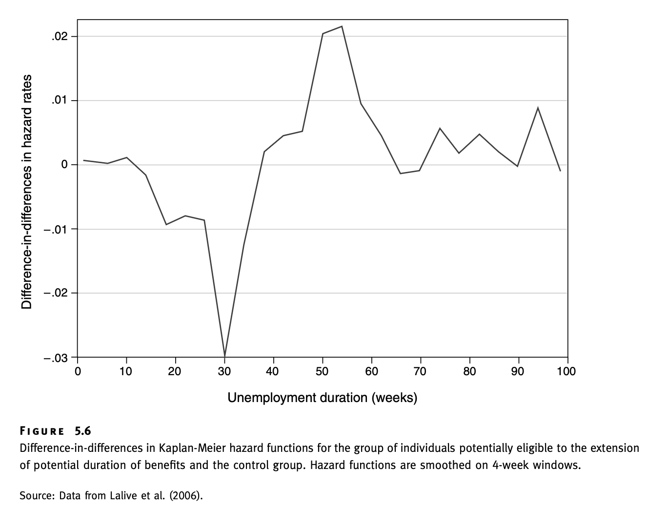
The figure shows difference-in-difference estimate of change in hazard rate (probability of exiting unemployment spell) due to \(ePBD\) reform.
- Notice that even though average duration of unemployment increases, the effect is non-monotonic over time
- Indeed, the probability of exiting from unemployment by \(t=30\) drops sharply. It is not surprising, since eligible workers can continue receiving benefits for another 9 or 22 weeks.
- We also see small bump in probability of exiting unemployment at 39 weeks and a larger hike at 52 weeks.
In summary, average duration of unemployment does not tell the whole story. Probability of exiting unemployment spell can vary over time (not necessarily in monotonic way)
Card, Chetty, and Weber (2007)
Exit unemployment \(\neq\) find a job
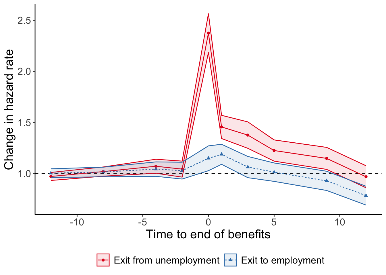
The outcome typically studied in the literature is duration of unemployment spell. But there are two ways that people can exit unemployment:
- find a new job (outcome of interest)
- stop looking for any jobs (might not be a desired outcome).
This is exactly what Card, Chetty, and Weber (2007) show. Also using Austrian data, they show that both types of exits from unemployment spike when benefits get exhausted. However, the spike in job finding rate is dwarfed by the spike in exit to non-employment!
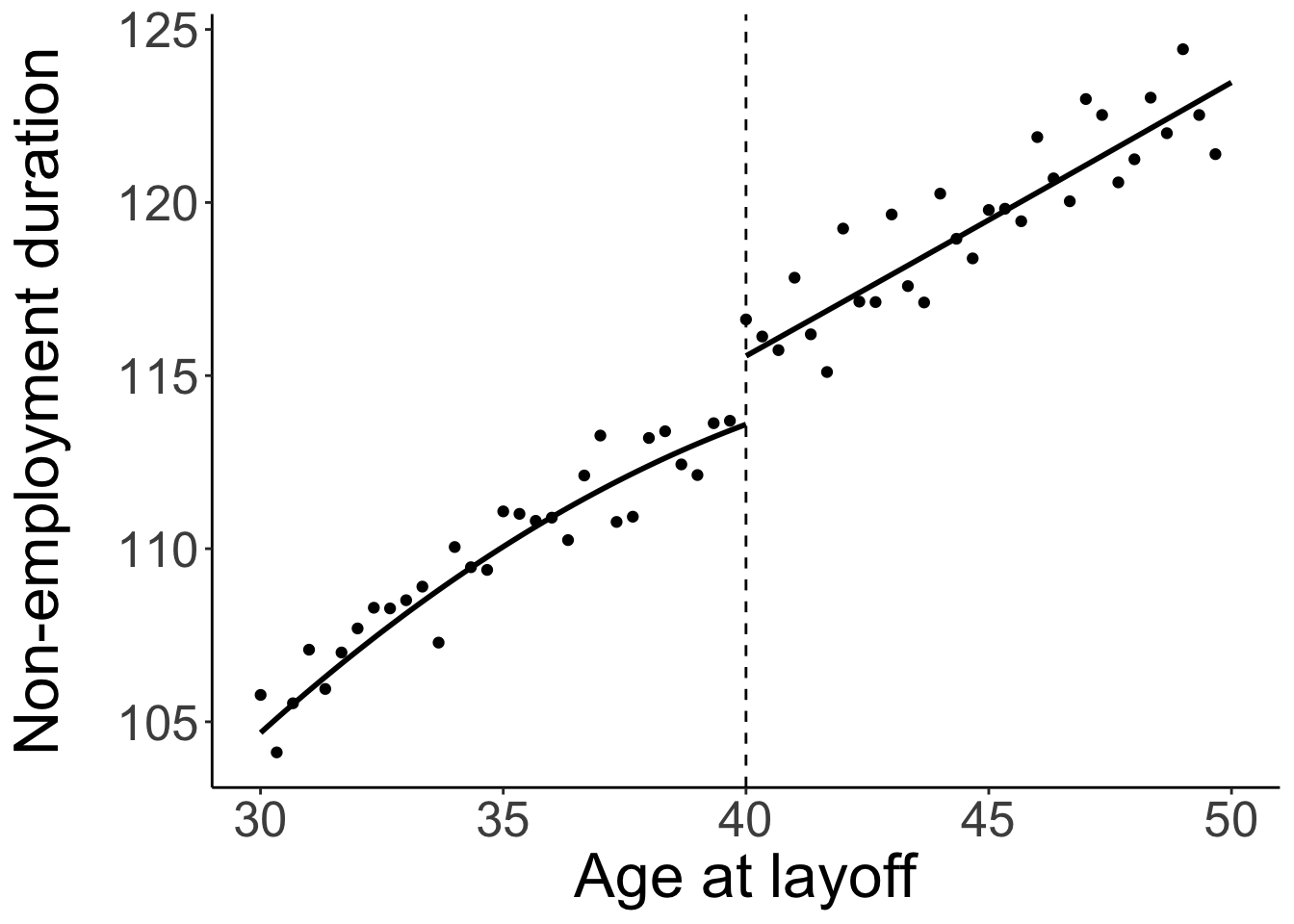
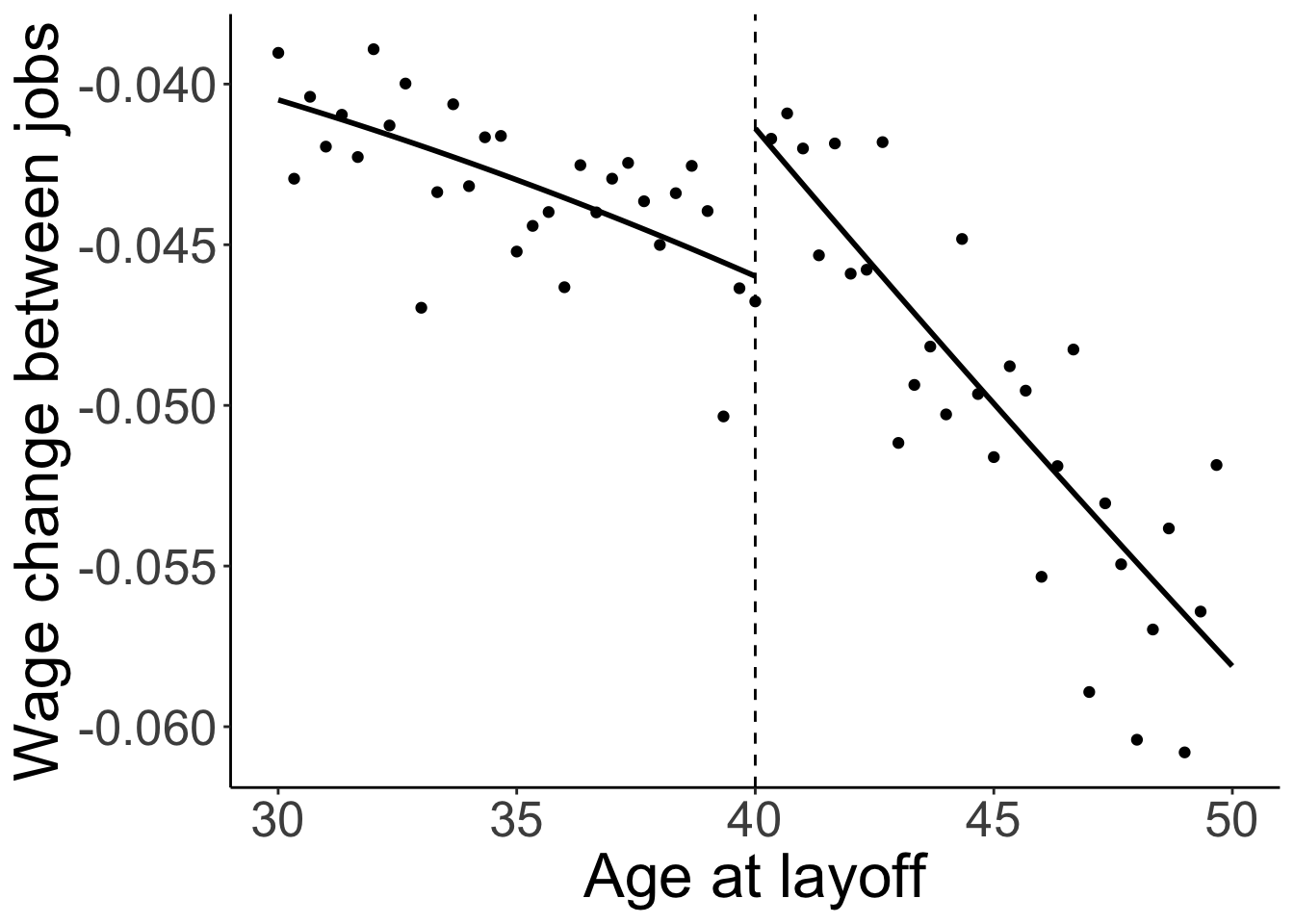
Nekoei and Weber (2017)
Generosity of benefits and quality of next job
- Regression discontinuity: compare Austrian workers around age 40
- Main finding: wage at next job \(\uparrow\)
- past papers: zero or \(<0\) effect
- Model: opposing forces on wages
- reservation wage \(\uparrow\)
- unemployment duration \(\uparrow\)
- Additional results:
- next job in higher-paying firms
- Policy impact:
- future tax revenue \(\uparrow\)
- current UI spending \(\uparrow\)
Simply finding a new job is only one facet of outcomes. Policy-makers and general society might also care about other characteristics of the new job. If people only care about finding jobs fast, they could lower their reservation wage and accept any job. However, if this job is a bad match for the skills of the worker, or personal preferences, it might not last long (so worker finds herself looking for jobs once again) and it would be inefficient allocation of labour force.
Nekoei and Weber (2017) study the relationship between unemployment benefits and the stability and wages at new jobs. They also use Austrian data with full information about unemployment spells. They use same policy change we’ve seen earlier: workers aged 40+ receive benefits for 9+ weeks longer.
This time, the authors use regression discontinuity design (RDD). The idea of this estimation method is following. You can rank people by their eligibility for a certain “treatment”. In this case, age determines the eligibility. Many policies specify a threshold after which individuals actually do receive “treatment”. In this case, the threshold is age 40. While people very far from thresholds are very different (20-year-olds behave differently from 60-year-olds), we can assume that people very close to the threshold are comparable (a 39-year-old behaves in same way as 41-year-old). This means that nothing else should “break” around the threshold, except only the receipt of “treatment” (benefits).
If you look at the top figure on the slide, you will see that consistent with the policy design, the probability of not working jumps at age 40. This is consistent with them receiving benefits for longer and not having to find a job soon. Now, instead of duration of unemployment spell you can use other outcomes (y axis) and see if they also jump at age 40. This is RDD in a nutshell. You can read more about it in Angrist and Pischke (2009).
Nekoei and Weber (2017) find significant and persistent positive effect of longer duration (more generous benefit) on wages at next job. However, this result seems to contradict past research that has found either zero or even negative effect of benefit generosity on future wages. To reconcile their findings with past literature, the authors use job search model with duration dependence. There are two opposing forces exerted on future wages
- We’ve seen already that more generous benefits raise the reservation wage.
- We’ve also seen that it increases unemployment duration, which in turn puts a downward pressure on reservation wages.
Therefore, depending on the strength of these two forces, the realised wages may change in either direction.
The additional results show that the increase in average wage at re-employment is largely due to matching to higher-paying firms (to all its workers). This is consistent with workers being able to keep searching for better matches (as opposed to having more bargaining power).
Belot, Kircher, and Muller (2019)
Cost of job search and re-employment
- Recommend vacancies based on skill set of jobseeker
- RCT: labs with computer access used for job search activity
- search for jobs in labs 1/week for 12 weeks
- weekly survey about interviews/offers and out-of-lab search
- on week 4, introduce recommendations to a random subsample
- Measure impact on
- breadth of occupations searched and applied for
- number of interviews
- job finding rate
Unemployment benefits are not the only way that policy-makers could affect job search behaviour of workers. Job search is costly to workers (and firms) and nature of this cost may be multi-dimensional. There can be financial costs: subscription to better job-search portals, travel to interviews, or acquisition of additional certificates. There can be cognitive costs: looking through many job ads, filtering bad and well-matched ads, tailoring applications, preparing for interviews, etc.
Advance of internet already lowered some of these costs significantly. People do not need to buy newspapers or walk around the town looking for job ads; simply log in to linkedin or headhunter. People don’t need to physically send their portfolios by mail or personally drop them in the offices; simply send the documents by email. Or even better, upload them on the portal, so potential employers could easily check them out themselves.
But internet also increased other costs. Now, workers and firms have to go through countless ads and applications just to find one job or candidate. So, they can overlook the well-matched options for various reasons.
Belot, Kircher, and Muller (2019) study focus on the issue that jobseekers might be looking for a very narrow set of job titles just because they don’t have enough information about other jobs. In particular, they might not know which other jobs their skills might be well-mathced to. The authors design an online tool that recommends a broader set of job postings where
- transferability of skills is high
- current labour market trends are favourable
They set up a randomised experiment where jobseekers are given computer access to a particular job search website. The jobseekers have to visit the computer lab once a week for 12 weeks. Besides recording their search behaviour inside the computer lab, they also ask them every week about applications, interviews and offers they received while searching on their own.
The crucial part is that the job search website offers wider range of jobs to a random subset of jobseekers. By randomising the group, they can ensure that people are not systematically selected based on their prior search behaviour or other characteristics.
Belot, Kircher, and Muller (2019)
| Dependent variable | ||||
|---|---|---|---|---|
| Breadth of applications | N applications | N interviews | N offers | |
| * p < 0.1, ** p < 0.05, *** p < 0.01 | ||||
| Treatment | 0.030 | 0.010 | 0.440* | -0.130 |
| (0.200) | (0.090) | (0.280) | (0.250) | |
| Treatment x init. broad | -0.430* | -0.050 | -0.070 | |
| (0.220) | (0.120) | (0.240) | ||
| Treatment x init. narrow | 0.490* | 0.080 | 1.030*** | 0.100 |
| (0.290) | (0.130) | (0.550) | (0.560) | |
| Num.Obs. | 305 | 487 | 464 | 253 |
In a similar experiment, Belot, Kircher, and Muller (2022) find
- \(\uparrow \Pr\) finding a stable job (at least 6 months)
- \(\uparrow \Pr\) reaching earnings threshold
The results in Belot, Kircher, and Muller (2019) suggest that recommending slightly wider set of occupations to jobseekers
- increases the breadth of jobs they apply for if they had been previously searching very narrowly
- does not increase number of applications they make (so it only changes composition of jobs they apply for)
- raises significantly number of interviews they have
- but seemingly does not result in successful offers.
However, the results on job finding rates should be taken with great caution due to small sample size. The job finding rates in the sample were already quite low (0.42 job offers on average). Given this low baseline level, the authors reckon that there should be at least 3 400 participants in treatment and control groups to be able to identify any treatment effect with statistical precision.
In a recent working paper, Belot, Kircher, and Muller (2022) provide similar occupational recommendations in the UK (also in an experimental setting) and measure outcomes at next job. The treatment increases probability of finding a stable job (i.e, one that lasts for at least 6 months or longer). It also increases the probability of reaching an earnings threshold (around £3 500). The threshold is computed as earnings of working for half a year 16 hours a week at minimum wage. Thus, the mere fact of reaching a threshold is not necessarily an indicator of high earnings. However, comparing the probability of reaching the threshold between the two groups (treatment and control) tells us something about their average earnings. Hence, earnings in the treatment group must be on average higher than in the control group. Therefore, the jobs that treated workers find after unemployment spell are generally better-paid than workers in the control group.
Summary
- Job search models labour supply under imperfect information
- Useful in studying unemployment spells and job search behaviour
- Accommodate firm side to characterise equilibrium wage distribution
- Useful in studying wage dispersion (more in next lecture)
- Necessary to assess full impact of policy change
- Empirical studies focus on
- effects of benefits on search behaviour
- duration dependence of search and job-finding rates
- effectiveness of various job search tools
Next lecture: Wage setting on 08 Sep
References
Angrist, Joshua David, and Jörn-Steffen Pischke. 2009. Mostly Harmless Econometrics: An Empiricist’s Companion. Princeton: Princeton University Press.
Belot, Michele, Philipp Kircher, and Paul Muller. 2019. “Providing Advice to Jobseekers at Low Cost: An Experimental Study on Online Advice.” The Review of Economic Studies 86 (4): 1411–47. https://doi.org/10.1093/restud/rdy059.
———. 2022. “Do the Long-Term Unemployed Benefit from Automated Occupational Advice During Online Job Search?” SSRN Electronic Journal. https://doi.org/10.2139/ssrn.4178928.
Cahuc, Pierre, Stéphane Carcillo, and André Zylberberg. 2014. Labor Economics. Second edition. Cambridge, MA: The MIT Press. https://research.ebsco.com/linkprocessor/plink?id=0949c8a9-3435-3a85-a9e3-d47d2c8a57ef.
Card, David, Raj Chetty, and Andrea Weber. 2007. “The Spike at Benefit Exhaustion: Leaving the Unemployment System or Starting a New Job?” The American Economic Review 97 (2): 113–18. https://www.jstor.org/stable/30034431.
Krueger, Alan B., and Andreas Mueller. 2010. “Job Search and Unemployment Insurance: New Evidence from Time Use Data.” Journal of Public Economics 94 (3): 298–307. https://doi.org/10.1016/j.jpubeco.2009.12.001.
Krueger, Alan B., and Andreas I. Mueller. 2012. “The Lot of the Unemployed: A Time Use Perspective.” Journal of the European Economic Association 10 (4): 765–94. https://doi.org/10.1111/j.1542-4774.2012.01071.x.
Lalive, Rafael, Jan van Ours, and Josef Zweimüller. 2006. “How Changes in Financial Incentives Affect the Duration of Unemployment.” The Review of Economic Studies 73 (4): 1009–38. https://www.jstor.org/stable/4123257.
McCall, J. J. 1970. “Economics of Information and Job Search.” The Quarterly Journal of Economics 84 (1): 113–26. https://doi.org/10.2307/1879403.
Mortensen, Dale T. 1970. “Job Search, the Duration of Unemployment, and the Phillips Curve.” The American Economic Review 60 (5): 847–62. https://www.jstor.org/stable/1818285.
Nekoei, Arash, and Andrea Weber. 2017. “Does Extending Unemployment Benefits Improve Job Quality?” American Economic Review 107 (2): 527–61. https://doi.org/10.1257/aer.20150528.
Official Statistics of Finland (OSF). 2025. “Time Use.” Online publication. https://stat.fi/en/statistics/akay.