8. Intergenerational mobility

KAT.TAL.322 Advanced Course in Labour Economics

Intergenerational mobility

Do children “inherit” their outcomes from parents?

Model of intergenerational mobility

Simplified Becker and Tomes (1979)

Budget constraint

Parent’s income $y_{t-1}$ allocated to consumption $C_{t-1}$ and investment into child $I_{t-1}$: $$y_{t-1}=C_{t-1}+I_{t-1}$$

Investment technology

Investment $I_{t-1}$ and other determinants $E_t$ produce child’s earnings $y_t$: $$y_t=(1+r)I_{t-1}+E_t$$

Maximise intergenerational utility (Cobb-Douglas)

$$\underset{I_{t-1},C_{t-1}}{max}(1-\alpha )\log C_{t-1}+\alpha \log y_t$$

$E_t$ are non-investment determinants (randomness?) that is known to the parent

Simplified Becker and Tomes (1979)

The first-order condition for $I_{t-1}$ implies

$$I_{t-1}=\alpha y_{t-1}-\frac{(1-\alpha )E_t}{1+r}$$

Plug it back to the investment technology equation:

$$y_t=\alpha (1+r)y_{t-1}+\alpha E_t$$

If $E_t\perp y_{t-1}$ and $Var(y_t)=Var(y_{t-1})\Rightarrow \text{Corr}(y_t,y_{t-1})=\alpha (1+r)$

Simplified Becker and Tomes (1979)

Intergenerational correlation

Suppose $E_t=e_t+u_t$, where $e_t$ is endowment and $u_t$ is randomness.

Endowment is passed down the generations: $e_t=\lambda e_{t-1}+v_t$

$$y_t=\alpha (1+r)y_{t-1}+\alpha e_t+\alpha u_t$$

Assuming $y_t$ is stationary,

$$\text{Corr}(y_t,y_{t-1})=\delta \alpha (1+r)+(1-\delta )\frac{\alpha (1+r)+\lambda }{1+\alpha (1+r)\lambda }$$

where $\delta =\frac{{\alpha }^2{\sigma }_u^2}{(1-{\alpha }^2(1+r{)}^2){\sigma }_y^2}$.

Together with explanations on the next slide, point out different components and build story.

Simplified Becker and Tomes (1979)

Intergenerational correlation

Even the simple model highlights important channels:

• Importance $\alpha$ of child’s future earnings on parent’s utility

• Return to investments $r$ (e.g., returns to education)

• Strength of intergenerational transmission of endowments $\lambda$

• Magnitude of market luck relative to endowment luck $\delta$

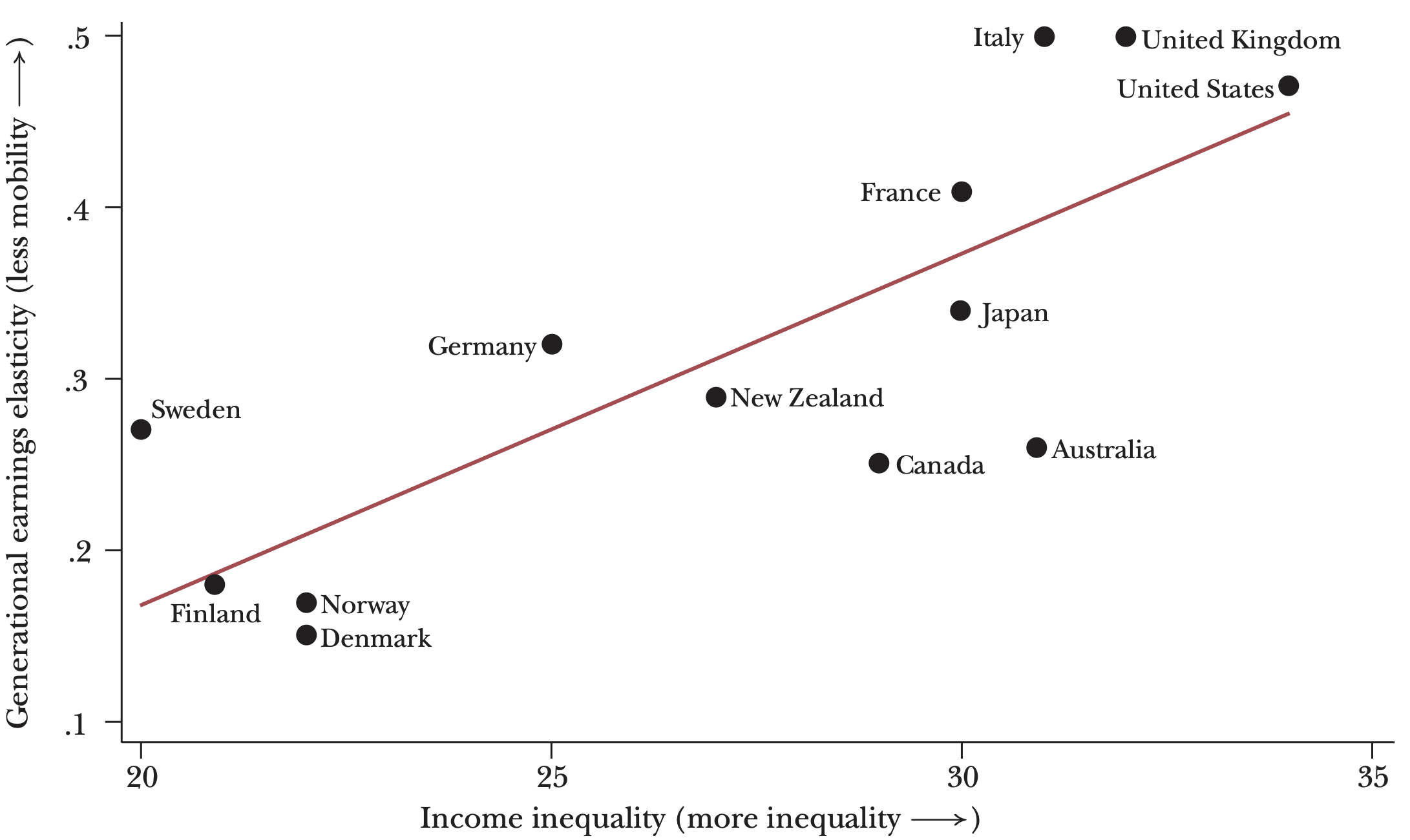
Notice $\uparrow r$ (a measure of income inequality) implies higher correlation between generations, or lower mobility.

This relationship is captured by the Great Gatsby curve.

The Great Gatsby curve

Source: Figure 1 in Corak (2013)

Simplified Becker and Tomes (1979)

Limitations

• Ignores transfer of assets (revisited Becker and Tomes 1986)

• Single parent $\Rightarrow$ ignores assortative mating

• Single child $\Rightarrow$ ignores intrahousehold allocation

• Arbitrary functional forms

  • For example, additive $I_{t-1}$ and $u_t$ imply offsetting
    Suppose, public investment $\uparrow \Rightarrow u_t\uparrow \Rightarrow I_{t-1}^{\star }\downarrow$
  • Data does not support (Head Start experiment)

Measurement

Basic framework

Simple regression (ignoring process on endowments)

$$y_t=\beta y_{t-1}+\epsilon$$

where $y_t$ and $y_{t-1}$ are log earnings and $\beta$ is IGE elasticity.

Challenges

• Data sources: cross-sectional, panel, retrospective?
• Permanent vs transitory earnings
• Measurement error
• Interpretation?

Measurement error

Source: Table 2 in Solon (1992)

Measurement error

Using father’s education as an instrument for father’s single-year earnings

 

Source: Table 4 in Solon (1992)

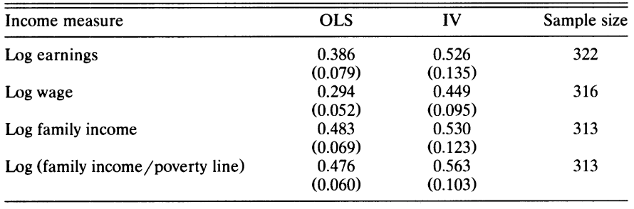
So, the idea is that by using an instrument, they can also approximate lifetime earnings potential even when using single-year measures

Permanent income

Source: Table 4 in Mazumder (2005)

Solon (1992) uses 5-year averages of income as “permanent”

However, transitory shocks can be persistent (unemployed today -> lower earnings next 5 years)

Therefore, 5-year averages contain both transitory and permanent components

Mazumder (2005) uses 15-year averages (administrative data linking)

Lifecycle bias

Haider and Solon (2006)

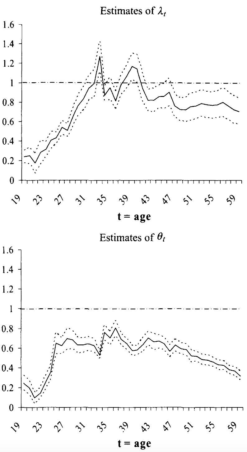
$$\begin{array}{rl}{y}_a^{\text{parent}}& ={\mu }_a{y}^{\text{parent}}+v\\ y_a^{\text{child}}& ={\lambda }_a{y}^{\text{child}}+u\end{array}$$

In this case, IGE elasticity estimator $\hat{\beta }$ is inconsistent:

$$\text{plim}\hat{\beta }=\beta {\lambda }_a{\theta }_a$$

where ${\theta }_a=\frac{{\mu }_a\text{Var}(y^{\text{parent}})}{{\mu }_a^2\text{Var}(y^{\text{parent}})+\text{Var}(v)}$

Intergenerational elasticity across countries

Jäntti et al. (2006)

	Men		Women
	Elasticity	Correlation	Elasticity	Correlation
Denmark	0.071	0.089	0.034	0.045
Finland	0.173	0.157	0.080	0.074
Norway	0.155	0.138	0.114	0.084
Sweden	0.258	0.141	0.191	0.102
UK	0.306	0.198	0.331	0.141
US	0.517	0.357	0.283	0.160

Source: Table 2

Mechanisms

Mechanisms

Black and Devereux (2011): recent studies focus on causal mechanisms

What is the “optimal” amount of intergenerational mobility?

Returns to skills

High $H$ parent invest more in child’s $H\Rightarrow$ high IG correlation

Unequal access

Type of policy depends on channel:

• public education/health
• democratic hiring policies
• …

Intergenerational mobility and education

Pekkarinen, Uusitalo, and Kerr (2009)

School reform in Finland 1972-77: selective $\to$ comprehensive

Source: Figure 1

The reforms also

• increased academic content of curriculum (more math and sciences)

• one foreign language became compulsory

$\Rightarrow$ new curriculum is

• more demanding for those who would have stayed in vocational track

• less demanding than in old secondary school! (because more heterogeneous students)

Plus, abolished private schools and imposed centralized control.

Intergenerational mobility and education

Pekkarinen, Uusitalo, and Kerr (2009)

Standard IGE elasticity regression

$$\begin{array}{}\text{(1)}& \log (y_{\text{son}})=a+b_{jt}\log (y_{\text{father}})+e\end{array}$$

Effect of reform on IGE elasticity

$$\begin{array}{}\text{(2)}& b_{jt}=b_0+\delta R_{jt}+\mathrm{\Omega }{D}_j+\mathrm{\Psi }{D}_t\end{array}$$

where $R_{jt}$ indicates if reform in municipality $j$ affected cohort $t$.

Substitute Eq 2 into Eq 1 + main effects

Source: Figure 2

Write out the full regression equation

$$\begin{array}{rl}\log (y_{\text{son}})=& a+b_0\log (y_{\text{father}})+\\ & +\delta R_{jt}\log (y_{\text{father}})+(\mathrm{\Omega }{D}_j+\mathrm{\Psi }{D}_t)\log (y_{\text{father}})+\\ & +\mathrm{\Phi }{D}_t+\mathrm{\Pi }{D}_j+\gamma R_{jt}+e_{ijt}\end{array}$$

Intergenerational mobility and education

Pekkarinen, Uusitalo, and Kerr (2009)

	(1)	(2)	(3)	(4)
Father’s earnings	0.277	0.297	0.298	0.296
	(0.014)	(0.011)	(0.010)	(0.014)
Reform		−0.063	−0.019
		(0.012)	(0.021)
Father’s earnings $\times$ reform		−0.055	−0.069	−0.066
		(0.009)	(0.022)	(0.031)
Obs.	20 824	20 824	20 824	20 824
$R^2$	0.05	0.05	0.05	0.06
Cohort FE			Yes	Yes
Father’s earnings $\times$ cohort FE			Yes	Yes
Region FE			Yes	Yes
Father’s earnings $\times$ region FE			Yes	Yes
Cohort FE $\times$ region FE				Yes
Region-specific trend				Yes

Source: Table 3

Last column add fully interacted FEs $\Rightarrow$ main effect of the reform is no longer identified

BUT interaction is still identified and is consistent with other columns!

Improving access to education promotes intergenerational mobility

Intergenerational spillovers in education

Do educational reforms have spillover effects on children?

Black, Devereux, and Salvanes (2005)

School reform in Norway in 1960-71: compulsory edu 7 $\to$ 9 years

IV approach

$$\begin{array}{rl}E& =\beta E^p+\gamma X+{\gamma }_p{X}^p+ϵ\\ E^p& =\alpha {REFORM}^p+\delta X+{\delta }_p{X}^p+v\end{array}$$

Source: Figure 1

Limited IG spillover of school reform at the bottom

Intergenerational spillovers in education

Suhonen and Karhunen (2019)

Expansion of Finnish university system in 1955-75

Source: Figure 1

The third map shows 1995 (mostly expansion in student numbers)

Intergenerational spillovers in education

Suhonen and Karhunen (2019)

University access measures based on distance from municipality of birth

Event study and IV approach

$$\begin{array}{rl}{E}_{ijmc}^c& ={\beta }_0+{\beta }_1{E}_{ijmc}^p+{\beta }_2{X}_{ijmc}+{\theta }_m+{\mu }_c+{\epsilon }_{ijmc}\\ E_{ijmc}^p& ={\alpha }_0+{\alpha }_1{UniAccess}_{ijmc}+{\alpha }_2{X}_{ijmc}+{\gamma }_m+{\delta }_c+{\vartheta }_{ijmc}\end{array}$$

$i$ - child, $j$ - parent, $m$ - parent birth municipality, $c$ - parent birth cohort.

Intergenerational spillovers in education

Suhonen and Karhunen (2019)

	Child's years of education
	Full sample			Grandparent nonmissing
	OLS	IV
	(1)	(2)	(3)	(4)
Mother-child sample
Mother's years of education	0.345***	0.522***	0.540***	0.697***
	(0.004)	(0.133)	(0.143)	(0.120)
F-stat (IV)		4.1	14.2	21.3
Obs.	1 239 331	1 239 331	1 239 331	628 230
Father-child sample
Father's years of education	0.305***	0.400**	0.535***	0.612***
	(0.003)	(0.161)	(0.171)	(0.143)
F-stat (IV)		3.7	12.7	19.6
Obs.	1 195 008	1 195 008	1 195 008	710 677
Additional controls			Yes	Yes

Source: Table 7

1 extra year of mother education leads to 0.5-0.6 year of child education

1 extra year of father education leads to 0.4-0.5 year of child education

the complier parents are mainly low-income and low-educated $\Rightarrow$ IG spillovers could lead to higher mobility of their children as well

Intergenerational spillovers in education

Suhonen and Karhunen (2019)

Strong positive spillover from parent’s to child’s education

Suggestive evidence that

• assortative mating between parents can account for >50% of effects

• higher parental income could also contribute to the results

• IG transmission present in pre-uni school outcomes

Important for mobility discussion: complier parents mainly from low-educated and low-income families

Intergenerational mobility and neighbourhoods

Chetty and Hendren (2018a)

IGE mobility varies geographically (Chetty et al. 2014)

Source: Figure II

Intergenerational mobility and neighbourhoods

Chetty and Hendren (2018a)

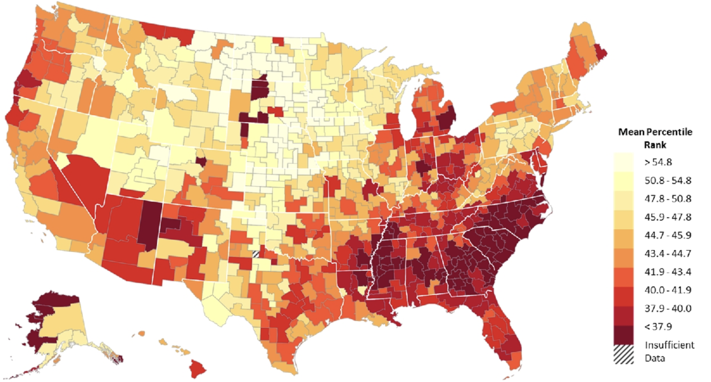
Geographic variation in IGE mobility may stem from:

• selection into neighbourhoods

• causal effect of neighbourhoods

Do children moving to higher mobility area have better outcomes?

Endogenous moving $\Rightarrow$ exploit timing of move

Identifying assumption

Selection into moving to a better area does not vary with age

Intergenerational mobility and neighbourhoods

Chetty and Hendren (2018a)

Source: Figure IV

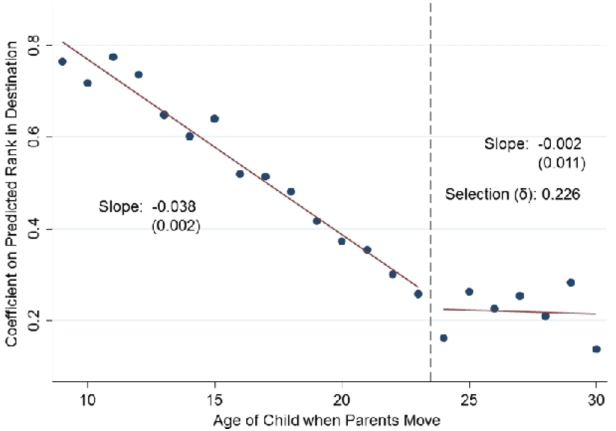
• Moving to a more mobile place improves success in proportion to exposure!

• children who move at age 9 would pick up 56% of the observed difference in permanent residents’ outcomes between their origin and destination CZs

• extrapolating: being born in a better area - pick up about 80% of the difference!

Intergenerational mobility and neighbourhoods

Chetty and Hendren (2018b)

What makes neighbourhoods generate good outcomes?

1. Segregation (maps)
   Racial and income segregation $\sim$ lower upward mobility
2. Income inequality
   “Areas with greater income inequality generate less upward mobility”
3. School quality
   $\uparrow$ test scores, $\downarrow$ school dropout rates, $\uparrow$ # of colleges per capita
4. Social capital
   $\uparrow$ participation in community activities, $\downarrow$ crime rate

Together explain 58% of variation in CZ causal effect

Social capital = participation in civic organiziations, bowling centers, golf clubs, fitness centers, sports organizations, religious organizations, political organizations, labour, business and professional organizations.

Intergenerational mobility and genetics

Rustichini et al. (2023)

How much of IGE elasticity driven by nature vs nurture?

Extension of standard model:

• genetic transmission and assortative mating

• skill transmission: genetic factors, parental investments, family environment and idiosyncratic events

Minnesota Twin Family Study (income, skills, genotypes + parents)

Intergnerational mobility and genetics

Rustichini et al. (2023)

Source: Table 1

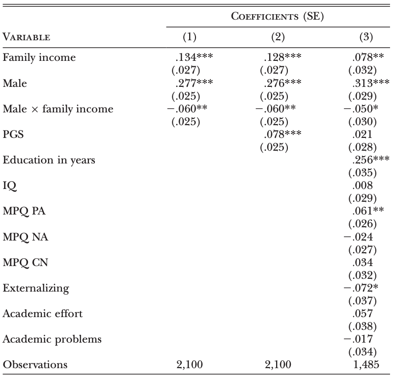
PGS as measure of genetic endowment affects significantly the income

• hence endowment plays an important role

• most of the PGS effect is mediated via education variables

• so, it is possible that PGS determines the investments they get

• also part of the PGS effect carries the weight of assortative mating

  • observed PGS correlation between twins - expected correlation = 0.083

Intergenerational mobility and genetics

Rustichini et al. (2023)

Source: Table 3

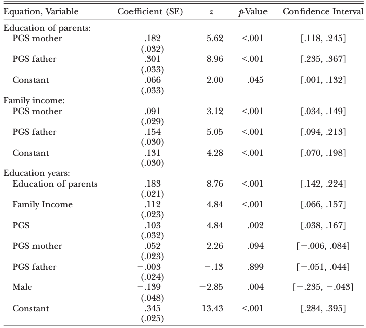
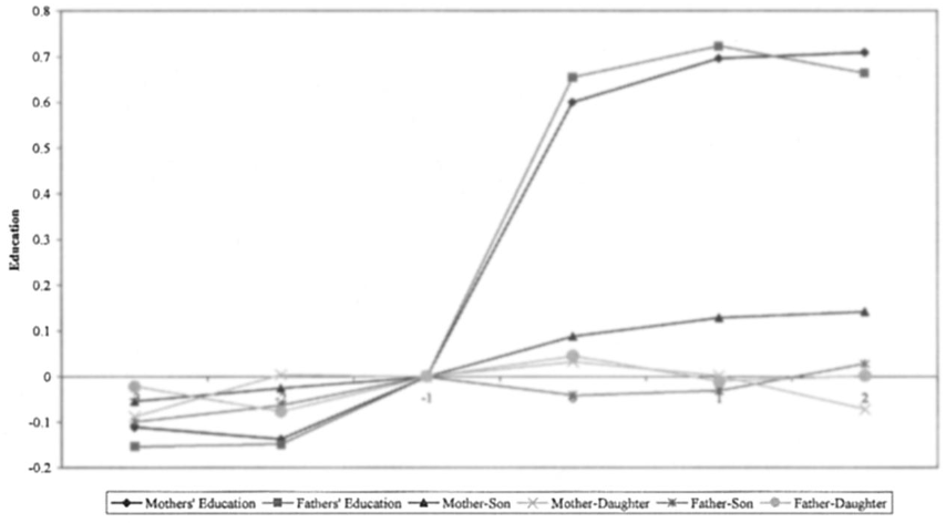
The last panel (equation of education years of children) shows that

• PGS of parents completely mediated through family environment variables such as parent education and family income

• PGS of child remains highly significant and large, so genetic endowment continue to play an important role

Multigenerational mobility

Colagrossi, d’Hombres, and Schnepf (2020)

Typical regression of parent-child pairs

$$\ln y^{\text{child}}={\beta }_{-1}\ln y^{\text{parent}}+\epsilon$$

Similar estimation across $k$ generations

$$\ln y^{\text{child}}={\beta }_{-k}\ln y^{k\text{ ancestor}}+\vartheta$$

Iterated regression fallacy: ${\beta }_{-k}\ne {\left({\beta }_{-1}\right)}^k$

Multigenerational mobility

Colagrossi, d’Hombres, and Schnepf (2020)

Source: Figure 2

Multigenerational mobility

Stuhler (2012)

Possible explanations of iterated regression fallacy:

Latent endowment

$$\begin{array}{rl}{y}_{it}& =\rho e_{it}+u_{it}\\ e_{it}& =\lambda e_{it-1}+v_{it}\\ \Rightarrow \mathrm{\Delta }& =({\rho }^2-1){\rho }^2{\lambda }^2\end{array}$$

Multiple endowments

$$\begin{array}{rl}{y}_{it}& ={\rho }_1{e}_{1it}+{\rho }_2{e}_{2it}+u_{it}\\ e_{1it}& ={\lambda }_1{e}_{1it-1}+v_{1it}\\ e_{2it}& ={\lambda }_2{e}_{2it-1}+v_{2it}\\ \Rightarrow \mathrm{\Delta }& =-{\rho }_1^2{\rho }_2^2{({\lambda }_1-{\lambda }_2)}^2\end{array}$$

Grandparent effect

$$e_{it}={\lambda }_{-1}{e}_{it-1}+{\lambda }_{-2}{e}_{it-2}+v_{it}$$

Other explanations

Parental investments, bequests, etc.

Multigenerational mobility

Barone and Mocetti (2021)

Current individuals in Florence $\leftrightarrow$ ancestors in 1427 based on surnames

Source: Table 3

Multigenerational mobility

Collado, Ortuño-Ortín, and Stuhler (2023)

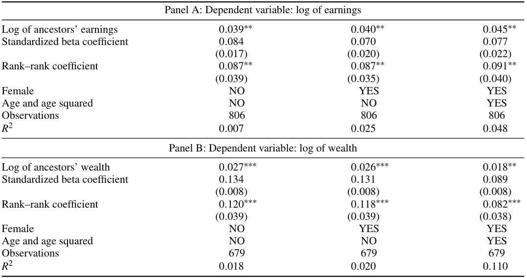
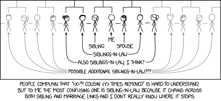
Horizontal approach: Grandparent-grandchild $\to$ cousin-cousin

• blood relationships: intergenerational processes

• in-law relationships: assortative processes

Swedish registry: “up to 141 distinct kinship moments”

Source: https://xkcd.com/2040

Multigenerational mobility

Collado, Ortuño-Ortín, and Stuhler (2023)

$$\begin{array}{rl}{y}_t& =\beta {\tilde{y}}_{t-1}+\gamma {\tilde{z}}_{t-1}+e_t+v_t+x_t+u_t\\ {\tilde{y}}_{t-1}& ={\alpha }_y{y}_{t-1}^m+(1-{\alpha }_y)y_{t-1}^f\\ {\tilde{z}}_{t-1}& ={\alpha }_z{z}_{t-1}^m+(1-{\alpha }_z)z_{t-1}^f\end{array}$$

$\beta$ and ${\alpha }_y$ measure direct transmission
$\gamma$ and ${\alpha }_z$ measure indirect transmission

$u_t$ is white noise (market luck)
$v_t$ is white noise in latent factor (endowment luck)
$x_t$ is shared sibling component
$e_t$ is latent sibling component

Multigenerational mobility

Collado, Ortuño-Ortín, and Stuhler (2023)

	$\beta$	$\gamma$	${\alpha }_y$	${\alpha }_z$	${\sigma }_y^2$	${\sigma }_u^2$	${\sigma }_z^2$	${\sigma }_x^2$	${\sigma }_e^2$
Men	0.144	0.664	0.389	0.660	4.648	1.975	2.072	0.180	0.657
Women	0.129	0.566	0.018	0.775	4.465	2.333	1.559	0.244	0.712

Figure 1: Source: Table 4

1. Indirect transmission dominates direct ($\beta <\gamma$)
2. Shared sibling component $x$ explains ~5%, $e$ ~ 15% of ${\sigma }_y^2$
3. Spousal correlation in latent factor > observed factor

Summary

• Vast literature on intergenerational mobility

  • Earlier works concentrated on measuring mobility precisely
  • Later works focus on determinants of mobility

• Improving access to education promotes mobility

  • The effect may spillover to children

• Geographic variation in mobility; largely causal

  • Lower segregation, inequality, better schools and social cohesion

• Genetic endowment and assortative mating important components

• Multigenerational mobility slower than predicted

References

Barone, Guglielmo, and Sauro Mocetti. 2021. “Intergenerational Mobility in the Very Long Run: Florence 1427–2011.” The Review of Economic Studies 88 (4): 1863–91. https://doi.org/10.1093/restud/rdaa075.

Becker, Gary S., and Nigel Tomes. 1979. “An Equilibrium Theory of the Distribution of Income and Intergenerational Mobility.” Journal of Political Economy 87 (6): 1153–89. https://www.jstor.org/stable/1833328.

———. 1986. “Human Capital and the Rise and Fall of Families.” Journal of Labor Economics 4 (3): S1–39. https://www.jstor.org/stable/2534952.

Black, Sandra E., and Paul J. Devereux. 2011. “Recent Developments in Intergenerational Mobility.” In Handbook of Labor Economics, 4:1487–1541. Elsevier. https://doi.org/10.1016/S0169-7218(11)02414-2.

Black, Sandra E., Paul J. Devereux, and Kjell G. Salvanes. 2005. “Why the Apple Doesn’t Fall Far: Understanding Intergenerational Transmission of Human Capital.” The American Economic Review 95 (1): 437–49. https://www.jstor.org/stable/4132690.

Chetty, Raj, and Nathaniel Hendren. 2018a. “The Impacts of Neighborhoods on Intergenerational Mobility I: Childhood Exposure Effects*.” The Quarterly Journal of Economics 133 (3): 1107–62. https://doi.org/10.1093/qje/qjy007.

———. 2018b. “The Impacts of Neighborhoods on Intergenerational Mobility II: County-Level Estimates*.” The Quarterly Journal of Economics 133 (3): 1163–1228. https://doi.org/10.1093/qje/qjy006.

Chetty, Raj, Nathaniel Hendren, Patrick Kline, and Emmanuel Saez. 2014. “Where Is the Land of Opportunity? The Geography of Intergenerational Mobility in the United States *.” The Quarterly Journal of Economics 129 (4): 1553–623. https://doi.org/10.1093/qje/qju022.

Colagrossi, Marco, Béatrice d’Hombres, and Sylke V Schnepf. 2020. “Like (Grand)parent, Like Child? Multigenerational Mobility Across the EU.” European Economic Review 130 (November): 103600. https://doi.org/10.1016/j.euroecorev.2020.103600.

Collado, M Dolores, Ignacio Ortuño-Ortín, and Jan Stuhler. 2023. “Estimating Intergenerational and Assortative Processes in Extended Family Data.” The Review of Economic Studies 90 (3): 1195–1227. https://doi.org/10.1093/restud/rdac060.

Corak, Miles. 2013. “Income Inequality, Equality of Opportunity, and Intergenerational Mobility.” Journal of Economic Perspectives 27 (3): 79–102. https://doi.org/10.1257/jep.27.3.79.

Gelber, Alexander, and Adam Isen. 2013. “Children’s Schooling and Parents’ Behavior: Evidence from the Head Start Impact Study.” Journal of Public Economics 101 (May): 25–38. https://doi.org/10.1016/j.jpubeco.2013.02.005.

Haider, Steven, and Gary Solon. 2006. “Life-Cycle Variation in the Association Between Current and Lifetime Earnings.” The American Economic Review 96 (4): 1308–20. https://www.jstor.org/stable/30034342.

Jäntti, Markus, Bernt Bratsberg, Knut Røed, Oddbjørn Raaum, Robin Naylor, Eva Österbacka, Anders Björklund, and Tor Eriksson. 2006. “American Exceptionalism in a New Light: A Comparison of Intergenerational Earnings Mobility in the Nordic Countries, the United Kingdom and the United States.” IZA Discussion Paper. Bonn, Germany. January 2006.

Mazumder, Bhashkar. 2005. “Fortunate Sons: New Estimates of Intergenerational Mobility in the United States Using Social Security Earnings Data.” The Review of Economics and Statistics 87 (2): 235–55. https://www.jstor.org/stable/40042900.

Pekkarinen, Tuomas, Roope Uusitalo, and Sari Kerr. 2009. “School Tracking and Intergenerational Income Mobility: Evidence from the Finnish Comprehensive School Reform.” Journal of Public Economics 93 (7): 965–73. https://doi.org/10.1016/j.jpubeco.2009.04.006.

Rustichini, Aldo, William G. Iacono, James J. Lee, and Matt McGue. 2023. “Educational Attainment and Intergenerational Mobility: A Polygenic Score Analysis.” Journal of Political Economy 131 (10): 2724–79. https://doi.org/10.1086/724860.

Solon, Gary. 1992. “Intergenerational Income Mobility in the United States.” The American Economic Review 82 (3): 393–408. https://www.jstor.org/stable/2117312.

Stuhler, Jan. 2012. “Mobility Across Multiple Generations: The Iterated Regression Fallacy.” SSRN Electronic Journal. https://doi.org/10.2139/ssrn.2192768.

Suhonen, Tuomo, and Hannu Karhunen. 2019. “The Intergenerational Effects of Parental Higher Education: Evidence from Changes in University Accessibility.” Journal of Public Economics 176 (August): 195–217. https://doi.org/10.1016/j.jpubeco.2019.07.001.

Appendices

Head Start and absence of offsetting behaviour

Source: Table 2 in Gelber and Isen (2013)

Back

US Racial Dot Map

Chicago

Sacramento

Figure 2: Source: US Census Bureau

Back

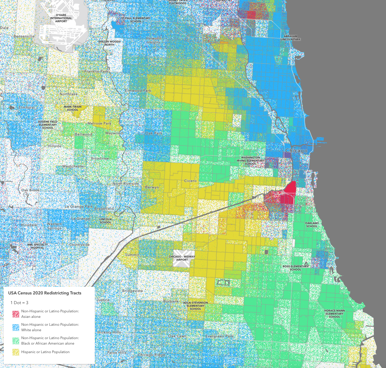
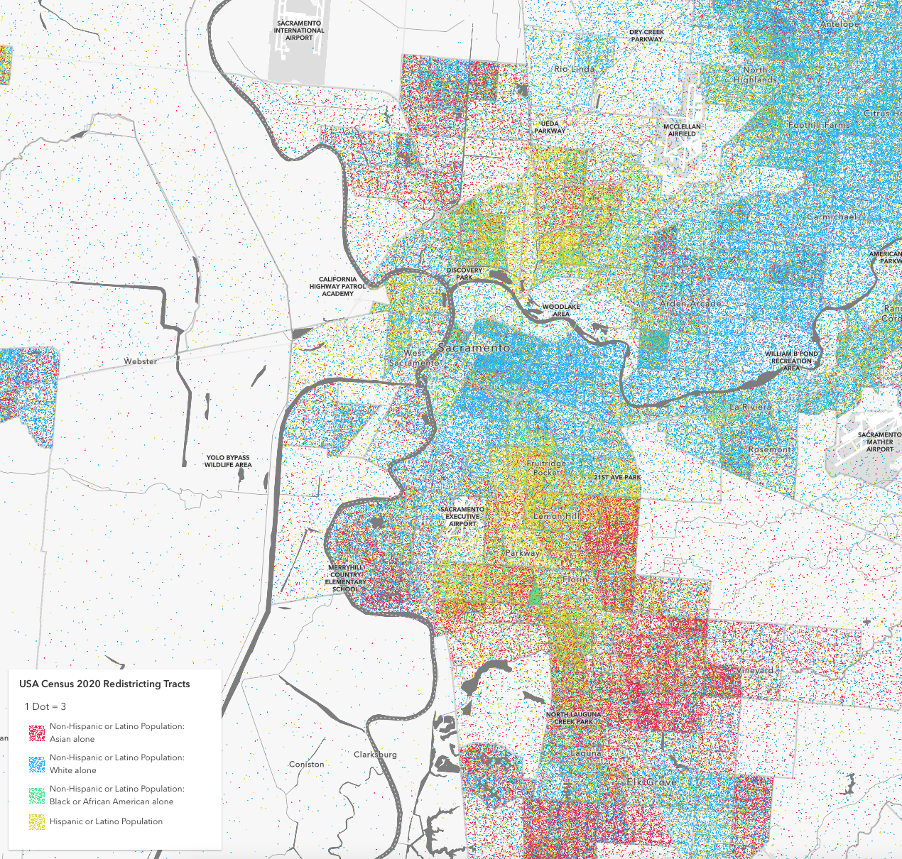
White - blue

Black - green

Asian - red

Hispanic - yellow