7. Labour market discrimination

KAT.TAL.322 Advanced Course in Labour Economics

Labour market discrimination

What is discrimination?

Discrimination arises when for the same level of productive characteristics, labour market outcomes differ based on nonproductive characteristics.

• Employers may discriminate in hiring/firing decisions

• Co-workers may discriminate in collaboration activity

• Customers may discriminate in purchase decisions

Taste discrimination

Taste discrimination

First formalized by Becker (1957)

• There are two types of workers $A$ and $B$
• Workers are perfect substitutes in production function $F(A+B)$
  $\Rightarrow$ equally productive $F_A(\cdot )=F_B(\cdot )$

A firm decides which worker to employ to maximise the utility

$$\underset{A,B}{max}PF(A+B)-w_{A}A-w_{B}B-dB$$

where $d\ge 0$ is the disutility employer gets from worker $B$.

• Emphasize that both workers have same effect on profit (free of discrimination)

• The disutility in this case has nothing to do with profit

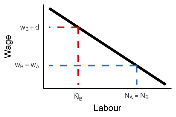
Taste discrimination

Optimal labour demand conditions

$$\begin{array}{rl}P{F}_A(A+B)& =w_A\\ P{F}_B(A+B)& =w_B+d\end{array}$$

Discriminating firm ($d>0$) hires $B$ workers iff $w_A>w_B+d$.

Employment of $B$ workers is lower than competitive level.

 

Taste discrimination

Perfect competition and free entry

Non-discriminating firms $d=0$ enters the market

Pay competitive wages to both groups $w_A=w_B=P{F}_L(L)$

Therefore,

• discriminating firms hire $A$ workers at $w_A$

• non-discriminating firms hire everyone at $w_A=w_B=w$

Taste discrimination cannot persist under perfect competition

• Discuss co-worker discrimination

  • perfect competition: workers are free to move to firms that do not hire the other worker type $\Rightarrow$ also can’t persist

• Everyone is paid their marginal product

Taste discrimination

Imperfect competition

1. Monopsonistic employer

   Lower wages and lower employment of discriminated group. The disadvantages persist as long as the employer does not compete with non- (or less) discriminating employers.

2. Market frictions (Black 1995)

   Job search costs can lead to lower wages and longer unemployment spells in discriminated group.

   • Existence of prejudiced employers lowers reservation wage.

   • Therefore, wages of discriminated workers at non-discriminating firms are also lower.

Statistical discrimination

Statistical discrimination

Overview

Unobservable characteristics or imperfect measures of productivity.

Consider two workers with identical unobserved productivity $F_A(\cdot )=F_B(\cdot )$ belonging to different groups $A$ and $B$.

The workers may give signals, such as education, past performance, etc. These are noisy measures of true productivities.

Employers may use average group characteristics to infer quality of signal and update their beliefs about workers.

The statistical discrimination may also change education decisions of groups and lead to persistent inequality among groups.

Statistical discrimination

Environment

Two types of workers: high $h^{+}>0$ and low $h^{-}=0$

Employers use costless test to get more information about workers:

• $Pr(\text{pass}|h^{+})=1$
• $Pr(\text{pass}|h^{-})=p$ where $p\in [0,1]$

Employers know the overall share of efficient workers $\pi (h^{+})\equiv \pi$.

$$Pr(h=h^{+}|\text{pass})=\frac{Pr(h=h^{+}\text{ and pass})}{Pr\left(\text{pass}\right)}=\frac{\pi }{\pi +p(1-\pi )}$$

Hence, wages of workers passing the test are

$$\mathbb{E}(\text{productivity}|\text{pass})=h^{+}\frac{\pi }{\pi +p(1-\pi )}$$

• This wage is paid regardless of true type to anyone who passes the test

• Wage is increasing in $\pi$. Conversely, if someone is of type $h^{+}$ but belongs to a group where $\pi$ is very low, then their wage is much lower.

• The wage is decreasing in the test error $p$. The less precise the test is, the lower are wages!

Statistical discrimination

Self-fulfilling prophecies

Workers choose education to $\underset{e}{max}U(w,e)=\underset{e}{max}w-e$

If $e=1\Rightarrow$ worker achieves productivity $h^{+}$; otherwise, $h^{-}$:

$$\begin{array}{rl}\mathbb{E}\left(w^{+}\right)& =h^{+}\frac{\pi }{\pi +p(1-\pi )}\\ \mathbb{E}\left(w^{-}\right)& =p{w}^{+}\end{array}$$

In equilibrium, $\pi$ is equal to share of workers investing into education.

Statistical discrimination

Self-fulfilling prophecies

Worker invests into education iff

$$w^{+}-1\ge p{w}^{+}\Rightarrow \pi \ge \frac{p}{(h^{+}-1)(1-p)}$$

Workers invest into education if employers belief $\pi$ is sufficiently high.

Statistical discrimination

Multliple equilibria and persistent inequalities

Source: Figure 8.11 in Cahuc (2004)

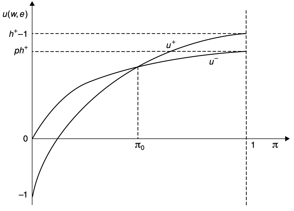
• If employers believe that $\pi =0$, there is no incentive to get educated $\Rightarrow$ everyone gets wage = 0
  • This can arise when testing is very imprecise such that too many uneducated people able to pass the test $p>\frac{h^{+}-1}{h^{+}}$. Then, the right hand side of the inequality on last slide is >1 and no $\pi$ can exceed it.
• If employers believe that $\pi =1$, then all workers want to get educated.
• There is some ${\pi }_0$ in the middle where all workers (since they are ex-ante identical) are indifferent between getting educated or not $\Rightarrow$ mixed strategy with ${\pi }_0=Pr(e=1)$
  • This equilibrium is unstable, because if employers believe $\pi +ϵ$ for some very small $ϵ>0$, then all workers get educated $\Rightarrow$ collapse to rightmost equilibrium with $\pi =1$
  • For $ϵ<0$, same argument leads to leftmost equilibrium with $\pi =0$
• Therefore, if employers believe that ${\pi }_A<{\pi }_0$ and ${\pi }_B>{\pi }_0$, then group A never gets education, group B always gets education and wage inequality between groups is very sticky!

Empirical results

Measuring discrimination

$\mathrm{\Delta }$ Wage by non-productive characteristics given same productivity.

Empirical challenges

• What constitutes a productive vs non-productive characteristic?

• Is $\mathrm{\Delta }$ wage attributable to discrimination alone or worker preferences?

• Does the discrimination arise from tastes or unobserved information?

Types of studies

• Observational

• Audit and correspondence studies

• Lab experiments

• Field experiments

• Quasi-random experiments

Kitagawa-Oaxaca-Blinder¹ decomposition

Wages in two groups ($A$ and $B$) can be written

$$\begin{array}{rl}\ln w_A& ={\mathbf{x}}_A{\mathit{\beta }}_A+{\epsilon }_A,\mathbb{E}\left({\epsilon }_A\right)=0\\ \ln w_B& ={\mathbf{x}}_B{\mathit{\beta }}_B+{\epsilon }_B,\mathbb{E}\left({\epsilon }_B\right)=0\end{array}$$

Then, average wage differential

$$\mathrm{\Delta }=\mathbb{E}(\ln w_A)-\mathbb{E}(\ln w_B)=[\mathbb{E}\left({\mathbf{x}}_A\right)-\mathbb{E}\left({\mathbf{x}}_B\right)]{\mathit{\beta }}_A+\mathbb{E}\left({\mathbf{x}}_B\right)({\mathit{\beta }}_A-{\mathit{\beta }}_B)$$

decomposed into explained and unexplained components.

Explained part is essentially composition effect.

Unexplained part: what would $B$ workers get if their returns were same as $A$’s?

The unexplained part on its own is not an evidence of discrimination!

Also show that decomposition is sensitive to the reference group!

Kitagawa-Oaxaca-Blinder decomposition

Interpretation

• Common support: ${\mathbf{x}}_A$ and ${\mathbf{x}}_B$ contain same set of variables
• Conditional mean independence: $\mathbb{E}({\epsilon }_A)=\mathbb{E}({\epsilon }_B)=0$
• Invariance of conditional distributions: distribution of ${\mathbf{x}}_B$ remains unchanged if $B$ workers receive returns ${\mathit{\beta }}_A$

These are very strict assumptions, so the decomposition is a correlational (not causal) measure.

Kitagawa-Oaxaca-Blinder decomposition

Source: Table 8.5 in Cahuc (2004)

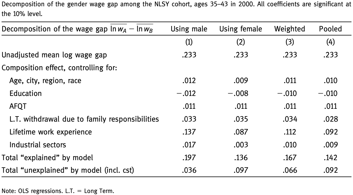
Point out the differences between different bases

Kitagawa-Oaxaca-Blinder decomposition over time

Blau and Kahn (1997): swimming upstream

$$\begin{array}{rl}{\mathrm{\Delta }}_t-{\mathrm{\Delta }}_s& =(\mathrm{\Delta }{X}_t-\mathrm{\Delta }{X}_s){\beta }_{At}+\mathrm{\Delta }{X}_s({\beta }_{At}-{\beta }_{As})+\\ & +(\mathbb{E}{x}_{Bt}-\mathbb{E}{x}_{Bs})\mathrm{\Delta }{\beta }_t+\mathbb{E}{x}_{Bs}(\mathrm{\Delta }{\beta }_t-\mathrm{\Delta }{\beta }_s)\end{array}$$

Total ${\mathrm{\Delta }}_t-{\mathrm{\Delta }}_s=-0.1522$ decomposed into (see Table 2)

1st term
2nd term
3rd term
4th term

Interpretation

Change in composition
Change in prices
Moving along distribution
Unexplained change

Contribution

-0.1244
0.0997
-0.1420
0.0143

Total wage differential fell by $\approx$ 15 percentage points.

The 4th term is crucial for the swimming upstream interpretation. If women did not move up along the distribution, i.e., their characteristics stayed at $\mathbb{E}{x}_{Bs}$, then the gender wage gap would have risen by 1.4pp.

Kitagawa-Oaxaca-Blinder decomposition

Summary

• Unexplained differences in earnings may be large (about 10%)

• They have also risen over time, so gender wage gap did not fall as much as it would have.

• But the unexplained differences $\ne$ discrimination

  • Selection into labour force, occupations, unobserved preferences
  • Counterfactual labour market returns can affect HC investments

Audit (correspondence) studies

• Send fictitious CVs nearly identical except in group membership

• Measure callback from firms or probability of getting interviews/offers

• RCT $\Rightarrow$ group differences can be interpreted as discrimination

Challenges

• CVs may not convey all relevant productive characteristics

• cannot disentangle taste discrimination from statistical

• hard to generalize to population

• focuses on mean differences, overlooks other moments

Remember that for statistical discrimination we want to get $\mathbf{\Delta }$ beliefs even if people are identical in every respect (observable and unobservable)

Therefore, if there are actual differences in unobservable characteristcs, it is not statistical discrimination, but correct economic decision!

• for CVs completeness:
  how can reflect great interpersonal skills or stress resilience other than face-to-face, probably repeated, interaction?

  • so, the group membership may convey some information about productive characteristics

• for generalization
  the total discrimination effect may be larger if people try to compensate by

  • sending out more CVs

  • being selective about firms

• for other moments
  Even if both groups are identical on average in observable and unobservable way, it can still be that unobservables are narrower in one group than the other. If employer knows that then the expected variance of unobservable distributions will also be picked up by the group dummy.

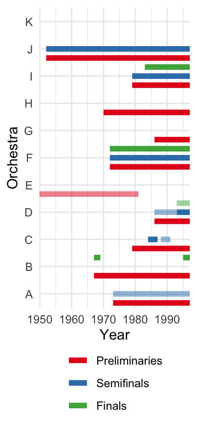
Goldin and Rouse (2000)

Before 1970s, musicians in orchestras were handpicked by the director

In 1970s-80s:

• auditions became more “open and routinized”
• musicians were hidden behind screen at some stage of audition

Staggered adoption of screen: difference-in-differences method

Auditions were advertised widely attracting 5x more applicants

Selection committee consisted of orchestra members, “not just conductor and section principal.”

Goldin and Rouse (2000)

Difference-in-differences approach

$$P_{ijtr}=\alpha +\beta F_i+\gamma B_{jtr}+\mathit{\delta }{F}_i\times B_{jtr}+X_{it}{\theta }_1+Z_{jtr}{\theta }_2+{\epsilon }_{ijtr}$$

$P_{ijtr}$ - prob $i$ advances in audition $j$ in year $t$ from round $r$
$F_i$ - gender
$B_{jtr}$ - indicator if screen is used
$X_{it}$ - other individual characteristics
$Z_{jtr}$ - other orchestral characteristics

Goldin and Rouse (2000)

Results

	Preliminaries
	Without semifinals	With semifinals	Semifinals	Finals
Female x Blind	0.111	−0.025	−0.235	0.331
	(0.067)	(0.251)	(0.133)	(0.181)
Obs.	5,395	6,239	1,360	1,127
R2	0.775	0.697	0.794	0.878

Source: Table 6

Bertrand and Mullainathan (2004)

Created templates for CVs of jobseekers in Boston and Chicago

• high and low quality types based on experience, skills, career profiles

• randomly assign distinctively White or African-American name

• track callback/email rates in race/sex/city/quality cell

	College degree	Years of experience	Volunteering experience?	Military experience?	E-mail address?	Employment holes?	Work in school?	Honors?	Computer skills?	Special skills?
White names	0.720	7.860	0.410	0.090	0.480	0.450	0.560	0.050	0.810	0.330
	(0.450)	(5.070)	(0.490)	(0.290)	(0.500)	(0.500)	(0.500)	(0.230)	(0.390)	(0.470)
African-American	0.720	7.830	0.410	0.100	0.480	0.450	0.560	0.050	0.830	0.330
	(0.450)	(5.010)	(0.490)	(0.300)	(0.500)	(0.500)	(0.500)	(0.220)	(0.370)	(0.470)

Source: Table 3

Bertrand and Mullainathan (2004)

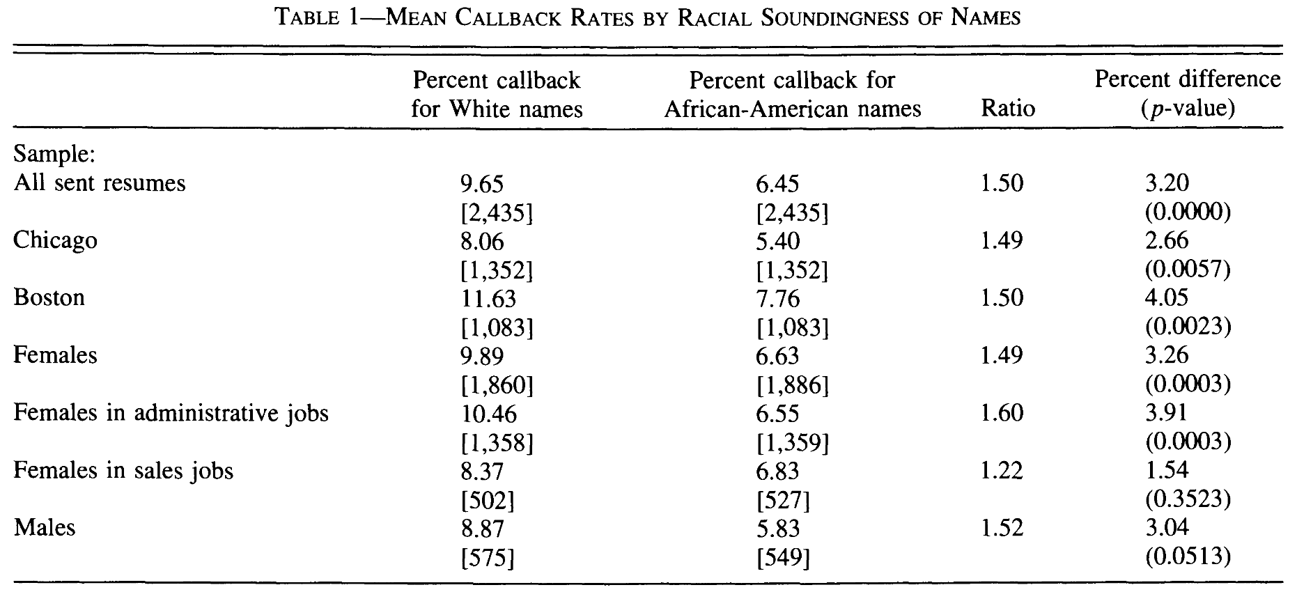
• Callback $\ne$ job offer or wage

• Race is only communicated via names
  There may be more discrimination once employers can see applicants. For example, not all African-Americans have distinct African-American names.

• Ignores other channels of job search (networks)

Mobius and Rosenblat (2006)

Lab experiment to measure taste discrimination based on beauty

Participants randomly assigned as workers (5) and employers (5).

1. Workers answer survey and solve simplest maze game

   Survey + practice time = digital CV

2. Workers predict # mazes solved in 15 min (private)

   $100A_j-40|C_j-A_j|$, where $A_j$ actual and $C_j$ predicted performance

   Measures confidence

Mobius and Rosenblat (2006)

3. Workers randomly matched to employers ($5\times 5$)

   B	CV only	(baseline)
   V	CV +	(visual)
   O	CV +	(oral)
   VO	CV + +	(visual and oral)
   FTF	CV + +	(face-to-face)

   1. Employers randomly told if their wage (next) adds to worker payoff

      Captures taste-based discrimination

4. Employers set wages $w_{ij}$ = # mazes could solve in 15 min

   ${\mathrm{\Pi }}_i=4000-40\sum _{j=1}^5|w_{ij}-A_j|$

Highlight the logic after the next slide!

an employer with taste for beauty might want to sacrifice earnings by giving higher $w_{ij}$. But if she knows her wages won’t affect the worker, she has no incentive to do so.

Mobius and Rosenblat (2006)

5. Workers complete 15 min “employment”

   The actual $A_j$s are realized.

6. Payoffs

   Firms receive ${\mathrm{\Pi }}_i$ as on previous slide
   Workers receive ${\mathrm{\Pi }}_j=100A_j-40|C_j-A_j|+\sum _{i=1}^5{W}_{ij}$ where $$W_{ij}=\{\begin{array}{ll}100w_{ij}& \text{with probability }80\mathrm{\%}\\ \overline{w}& \text{with probability }20\mathrm{\%}\end{array}$$

Mobius and Rosenblat (2006)

Results

1. Beauty does not affect actual performance, but increases confidence

2. There are beauty premia, but no evidence of taste-based discrimination

   	B	V	O	VO	FTF
   BEAUTY	0.017	0.131**	0.129**	0.124**	0.167**
   	(0.040)	(0.042)	(0.034)	(0.036)	(0.043)
   SETWAGE	−0.010	−0.072	0.098*	−0.046	0.033
   	(0.055)	(0.052)	(0.046)	(0.048)	(0.057)
   SETWAGE x BEAUTY	−0.058	−0.099+	0.005	−0.022	−0.044
   	(0.057)	(0.053)	(0.048)	(0.050)	(0.058)
   N	163	161	163	162	163

   Source: Table 4

3. 15-20% of beauty premium due to confidence, 40% due to stereotype

Stereotype = beauty making a worker appear more able in eyes of employers

Rao (2019)

Field and lab experiments eliciting taste-based discrimination

Policy change in India: elite schools required to offer free places to poor students. Staggered implementation $\Rightarrow$ diff-in-diff estimation

Results

• exposure to poor classmates makes students more prosocial
• it also reduces discrimination (teammate choices in race)
  • when stakes (prizes) are high, only 6% choose slower rich student over faster poor student
  • when stakes are low, 33% discriminate against poor students
  • past exposure $\downarrow$ taste discrimination WTP by 12pp

The prosocial effect is really driven by changes in fundamental notions of fairness and generosity.

Doleac and Hansen (2020)

Quasi-random policy experiment measuring statistical discrimination

Ban-the-box (BTB) policy

• Banning prior criminal convictions box on job applications
• Hawaii in 1998 $⟶$ 34 states + DC in 2015

BTB “does nothing to address the average job readiness of ex-offenders”.

Therefore, statistical discrimination may $\uparrow$

Use diff-in-diff to measure effect of BTB on employment of minorities

Obama banned the box in federal job applications in 2015

Doleac and Hansen (2020)

Results

	Full sample	BTB-adopting
White x BTB	−0.003	−0.005
	(0.006)	(0.008)
Black x BTB	−0.034**	−0.031**
	(0.015)	(0.014)
Hispanic x BTB	−0.023*	−0.020
	(0.013)	(0.015)
Obs.	503,419	231,933
Pre-BTB baseline
White	0.8219	0.8219
Black	0.677	0.677
Hispanic	0.7994	0.7994

Source: Table 4

Glover, Pallais, and Pariente (2017)

Capturing self-fulfilling prophecy of statistical discrimination

Quasi-random assignment of new cashiers to managers in French stores

Do minority cashiers perform worse with biased managers?

Measure manager bias using Implicit Association Test (IAT)

• 66% moderate to severe bias
• 20% slight bias

Outcomes: absences, time worked, scanning speed, time between customers

Minority = North or Sub-Saharan Africans (25-29% of new cashiers)

Glover, Pallais, and Pariente (2017)

Results

	Absences	Overtime (min)	Scan per min	Inter-customer time (sec)
Minority x Mngr bias	0.012***	−3.237*	−0.249**	1.360**
	(0.004)	(1.678)	(0.111)	(0.665)
Obs.	4,371	4,163	3,601	3,287
Dep var mean	0.0162	-0.068	18.53	28.7

Sources: Tables III and IV

Similarly, Carlana (2019)

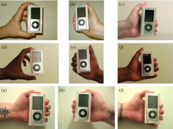
Doleac and Stein (2013)

Customer discrimination

Post ads selling iPods on 300 geographically local online markets

Black sellers get:

• 18% fewer offers

• $5.72 (11%) lower avg offer

• $7.07 (12%) lower best offer

Similar (sometimes larger) effect for tattooed

Source: Figure 1

Summary

• Two main frameworks with different implications for labour markets

  • Taste-based discrimination
  • Statistical discrimination

• Simple decomposition to measure unexplained gap and its changes over time

• Vast experimental and quasi-experimental literature

Next: Intergenerational mobility

References

Becker, Gary S. 1957. The Economics of Discrimination. Economic Research Studies. Chicago, IL: University of Chicago Press. https://press.uchicago.edu/ucp/books/book/chicago/E/bo22415931.html.

Bertrand, Marianne, and Sendhil Mullainathan. 2004. “Are Emily and Greg More Employable Than Lakisha and Jamal? A Field Experiment on Labor Market Discrimination.” The American Economic Review 94 (4): 991–1013. https://www.jstor.org/stable/3592802.

Black, Dan A. 1995. “Discrimination in an Equilibrium Search Model.” Journal of Labor Economics 13 (2): 309–34. https://www.jstor.org/stable/2535106.

Blau, Francine D., and Lawrence M. Kahn. 1997. “Swimming Upstream: Trends in the Gender Wage Differential in the 1980s.” Journal of Labor Economics 15 (1): 1–42. https://www.jstor.org/stable/2535313.

Cahuc, Pierre. 2004. Labor Economics. Cambridge (Mass.): MIT Press.

Carlana, Michela. 2019. “Implicit Stereotypes: Evidence from Teachers’ Gender Bias*.” The Quarterly Journal of Economics 134 (3): 1163–1224. https://doi.org/10.1093/qje/qjz008.

Doleac, Jennifer L., and Benjamin Hansen. 2020. “The Unintended Consequences of ‘Ban the Box’: Statistical Discrimination and Employment Outcomes When Criminal Histories Are Hidden.” Journal of Labor Economics 38 (2): 321–74. https://doi.org/10.1086/705880.

Doleac, Jennifer L., and Luke C. D. Stein. 2013. “The Visible Hand: Race and Online Market Outcomes.” The Economic Journal 123 (572): F469–92. https://www.jstor.org/stable/42919259.

Glover, Dylan, Amanda Pallais, and William Pariente. 2017. “Discrimination as a Self-Fulfilling Prophecy: Evidence from French Grocery Stores.” The Quarterly Journal of Economics 132 (3): 1219–60. https://www.jstor.org/stable/26372702.

Goldin, Claudia, and Cecilia Rouse. 2000. “Orchestrating Impartiality: The Impact of "Blind" Auditions on Female Musicians.” The American Economic Review 90 (4): 715–41. https://www.jstor.org/stable/117305.

Mobius, Markus M., and Tanya S. Rosenblat. 2006. “Why Beauty Matters.” The American Economic Review 96 (1): 222–35. https://www.jstor.org/stable/30034362.

Oaxaca, Ronald L., and Eva Sierminska. 2023. “Oaxaca-Blinder Meets Kitagawa: What Is the Link?” SSRN Electronic Journal. https://doi.org/10.2139/ssrn.4464602.

Rao, Gautam. 2019. “Familiarity Does Not Breed Contempt: Generosity, Discrimination, and Diversity in Delhi Schools.” American Economic Review 109 (3): 774–809. https://doi.org/10.1257/aer.20180044.

Footnotes

1. Formerly, Oaxaca-Blinder (Oaxaca and Sierminska 2023)