3. Labour Demand

KAT.TAL.322 Advanced Course in Labour Economics

Labour demand

Firm decisions about how much labour to hire.

Organizational bits:

1. Form groups on Moodle (demonstration)
   1. Group membership according to prior agreement with everyone in the group

Static model

Static model

Single factor input

Production function $Y=F(L)$ where $F^{\prime }>0$ and $F^{\prime \prime }<0$

$$\underset{L}{max}PF(L)-WL$$

FOC: $F^{\prime }(L)=\frac{W}{P}$

Downward-sloping labour demand $\frac{\partial L}{\partial W}=\frac{1}{P{F}^{\prime \prime }(L)}<0$

See Cahuc (2004) chapter 2 for similar non-competitive firm problem

• Labour is the only production input

• Increasing and concave production function

• Price-taking firm

• Knowing functional form of $F(\cdot )$ gives as labour demand function

Labour only $\approx$ short run (+ capital $\approx$ long run)

Static model

Two factor inputs: conditional factor demand

Cost minimization problem

$\underset{L,K}{min}C(L,K)=WL+RK$ s.t. $F(L,K)=\overline{Y}$

Conditional demand functions $\overline{K}(W,R,Y)$ and $\overline{L}(W,R,Y)$

$$\frac{F_L(\overline{L},\overline{K})}{F_K(\overline{L},\overline{K})}=\frac{W}{R}\text{and}F(\overline{L},\overline{K})=\overline{Y}$$

• $\frac{F_L(L,K)}{F_K(L,K)}$ is technical rate of substitution between capital and labour

• Draw the isoquant and isocost curves

Static model

Two factor inputs: conditional demand elasticities

• Own-price elasticities: ${\eta }_W^L=\frac{\partial \ln \overline{L}}{\partial \ln W}<0$, ${\eta }_R^K=\frac{\partial \ln \overline{K}}{\partial \ln R}<0$

• Cross-price elasticities: ${\eta }_R^L=\frac{\partial \ln \overline{L}}{\partial \ln R}>0$ and ${\eta }_W^K=\frac{\partial \ln \overline{K}}{\partial \ln W}>0$

• Elasticity of substitution $\sigma =\frac{\partial \ln \left(\frac{K}{L}\right)}{\partial \ln \left(\frac{W}{R}\right)}>0$

It is also possible to show that

$${\eta }_R^L=\sigma (1-s)\text{and}{\eta }_W^L=-\sigma (1-s)$$

where $s=\frac{WL}{C}$ is labour share in total cost

Derivations in Cahuc (2004) chapter 2

• Own-price elasticities always negative again due to concavity of the production function (intuitive)

• Cross-price elasticities are positive: with output fixed, if one factor is more expensive, substitute to the cheaper factor to offset.

  • Also intuitive, BUT do not tell to what extent substitution makes sense

• Therefore, elasticity of substitution

  • The sign is determined by the properties of cost function => direct to more detailed discussion in Cahuc (2004)

  • The positive sign in a sense is similar to cross-price intuition.

• The factor share expressions

  • useful empirically

  • alternative (easy) reasoning

Static model

Two factor inputs: unconditional factor demand

$\underset{Y}{max}PY-C(W,R,Y)$

Solution: $P=C_Y(W,R,Y^{\ast }),L^{\ast }=\overline{L}(W,R,Y^{\ast }),K^{\ast }=\overline{K}(W,R,Y^{\ast })$

Total elasticities decomposed into substitution and scale effects:

$${\epsilon }_W^L={\eta }_W^L+{\eta }_Y^L{\epsilon }_W^Y<0$$

$${\epsilon }_R^L={\eta }_R^L+{\eta }_Y^L{\epsilon }_R^Y\lessgtr 0$$

Similar conclusions in models with >2 inputs (Cahuc 2004, chap. 2, section 1.4)

• Now that we know minimum cost for every level of $Y$, only find $Y$ that maximizes profit

• $Y^{\star }$ given by first FOC $\Rightarrow$ $K^{\star }$ and $L^{\star }$ found by plugging $Y^{\star }$ to conditinal demands

• Now, can talk about total elasticity, substituion and scale.

• Encourage to go through derivations on their own!

• Own-price total elasticity (walk-through):

  • conditional elasticity ${\eta }_W^L<0$

  • scale: $\uparrow W\Rightarrow \downarrow Y\Rightarrow \downarrow L$ (homogeneous production function)

• Cross-price total elasticity:

  • do not walk through!

  • gross complements ${\epsilon }_R^L<0$ or gross substitutes ${\epsilon }_R^L>0$

$$\begin{array}{rl}\frac{\partial L^{\ast }}{\partial W}& =C_{WW}+C_{WY}\frac{\partial Y^{\ast }}{\partial W}=\\ & =C_{WW}+C_{WY}(-\frac{-C_{WY}}{-C_{YY}})=\\ & =C_{WW}+\frac{C_{WY}^2}{-C_{YY}}\end{array}$$

The sign of scale effect is then determined by the sign of $-C_{YY}$. A necessary condition for profit function to have a maximum is SOC < 0 $\Rightarrow -C_{YY}<0\Rightarrow$ scale effect is negative.

$$\begin{array}{rl}\frac{\partial L^{\ast }}{\partial R}& =C_{WR}+C_{WY}\frac{\partial Y^{\ast }}{\partial R}=\\ & =C_{WR}+C_{WY}(-\frac{-C_{RY}}{-C_{YY}})=\\ & =C_{WR}+\frac{C_{WY}{C}_{RY}}{-C_{YY}}\end{array}$$

Here the sign of the scale effect depends on signs of $C_{WY}$ and $C_{RY}$ which really depends on the production function.

Estimations of static model

Empirical strategy

Shephard’s lemma: specify cost function and back out labour demand

Example: translog cost function with $n$ inputs

$$\ln C=a_0+\sum _{i=1}^n{a}_i\ln W^i+\frac{1}{2}\sum _{i=1}^n\sum _{j=1}^n{a}_{ij}\ln W^i\ln W^j+\frac{1}{\theta }\ln Y$$

$$\Rightarrow s^i=a_i+\sum _{j=1}^n{a}_{ij}\ln W^j$$

Estimate parameters $a_i,a_{ij}$ and calculate implied elasticities.

Shephard’s lemma: $\overline{L}=\frac{\partial C}{\partial W}$ (keep $Y$ fixed)

$$L^i=\frac{\partial C}{\partial W^i}\Rightarrow \frac{W^i{L}^i}{C}=\frac{W^i}{C}\frac{\partial C}{\partial W^i}=W^i\frac{\partial \ln C}{\partial W^i}$$

Can get data about $s^i$ and $W^i$ directly $\Rightarrow$ estimate the share equation

Estimations of static model

Main issues

• Endogeneity

• General equilibrium

• Definitions of variables

Endogeneity:

• most productive firms hire more people and pay higher wages (cross-section)

• common shock that changes wages and employment, like trade shock (time-series)

Definition:

• how to measure labour: number of people, people hours, quality of labour

• wages: what about nonwage benefits that matter for firm decisions?

Estimations of static model

Review by Hamermesh (1996) concludes that $-{\eta }_W^L\in [0.15,0.75]$.

If ${\eta }_W^L=-0.30$ and given that $s\approx 0.7$,

$$\sigma =\frac{-{\eta }_W^L}{1-s}\approx 1$$

consistent with the Cobb-Douglas production function.

The review also suggests $-{\epsilon }_W^L\approx 1\Rightarrow$ large scale effect.

Dynamic model

Dynamic model

Adjustment costs

Share of non-wage labour costs

• Quadratic cost: $C\left(\mathrm{\Delta }{L}_t\right)=b{(\mathrm{\Delta }{L}_t-a)}^2$

• Assymmetric convex costs: $C\left(\mathrm{\Delta }{L}_t\right)=-1+e^{a\mathrm{\Delta }{L}_t}-a\mathrm{\Delta }{L}_t+\frac{b}{2}{\left(\mathrm{\Delta }{L}_t\right)}^2$

• Linear cost: $C\left(\mathrm{\Delta }{L}_t\right)=\{\begin{array}{ll}{c}_h\mathrm{\Delta }{L}_t& \text{if }\mathrm{\Delta }{L}_t\ge 0\\ -c_f\mathrm{\Delta }{L}_t& \text{if }\mathrm{\Delta }{L}_t\le 0\end{array}$

• Fixed cost

Examples of “adjustment” costs:

First ask them!

• costs associated with hiring/firing, maybe even promoting people

• but also nonwage benefits, such as extra healthcare insurance or lunch programs

Dynamic model

Quadratic adjustment cost

Continuous time $\Rightarrow \mathrm{\Delta }{L}_t={\dot{L}}_t=\frac{\text{d}{L}_t}{\text{d}t}$

$${\mathrm{\Pi }}_0={\int }_0^{\mathrm{\infty }}{\mathrm{\Pi }}_{t}dt={\int }_0^{\mathrm{\infty }}[F(L_t)-W_t{L}_t-\frac{b}{2}{\dot{L}}_t^2]e^{-rt}dt$$

Euler equation: $\frac{\partial {\mathrm{\Pi }}_t}{\partial L}=\frac{\text{d}}{\text{d}t}\left(\frac{\partial {\mathrm{\Pi }}_t}{\partial {\dot{L}}_t}\right)\Rightarrow b{\ddot{L}}_t-rb{\dot{L}}_t+F^{\prime }(L_t)-W_t=0$

Walk-through the derivation steps!

Euler condition derived in Cahuc (2004) (general result, take as given here)

$$\frac{\partial {\mathrm{\Pi }}_t}{\partial L_t}=(F^{\prime }(L_t)-W_t)e^{-rt}$$

$$\frac{\partial {\mathrm{\Pi }}_t}{\partial {\dot{L}}_t}=-b{\dot{L}}_t{e}^{-rt}$$

$$\frac{\partial }{\partial t}\left(\frac{\partial {\mathrm{\Pi }}_t}{\partial {\dot{L}}_t}\right)=-b{\ddot{L}}_t{e}^{-rt}+b{\dot{L}}_t{e}^{-rt}r$$

Therefore, plugging into Euler equation we get

$$(F^{\prime }(L_t)-W_t+b{\ddot{L}}_t-rb{\dot{L}}_t)e^{-rt}=0$$

Hence, the optimality condition on the slide.

1. Stationary solution ${\dot{L}}_t={\ddot{L}}_t=0\Rightarrow F^{\prime }(L_t)=W_t$
2. Inadequate if ${\dot{L}}_t=0$ achieved by hiring exactly offsetting firing

Dynamic model

Quadratic adjustment cost

Optimal path: ${\dot{L}}_t=\gamma [L^{\ast }-L_t]$ where $\gamma$ is decreasing in $b$.

Figure 9.6 Optimal employment over a cycle (Nickell 1986)

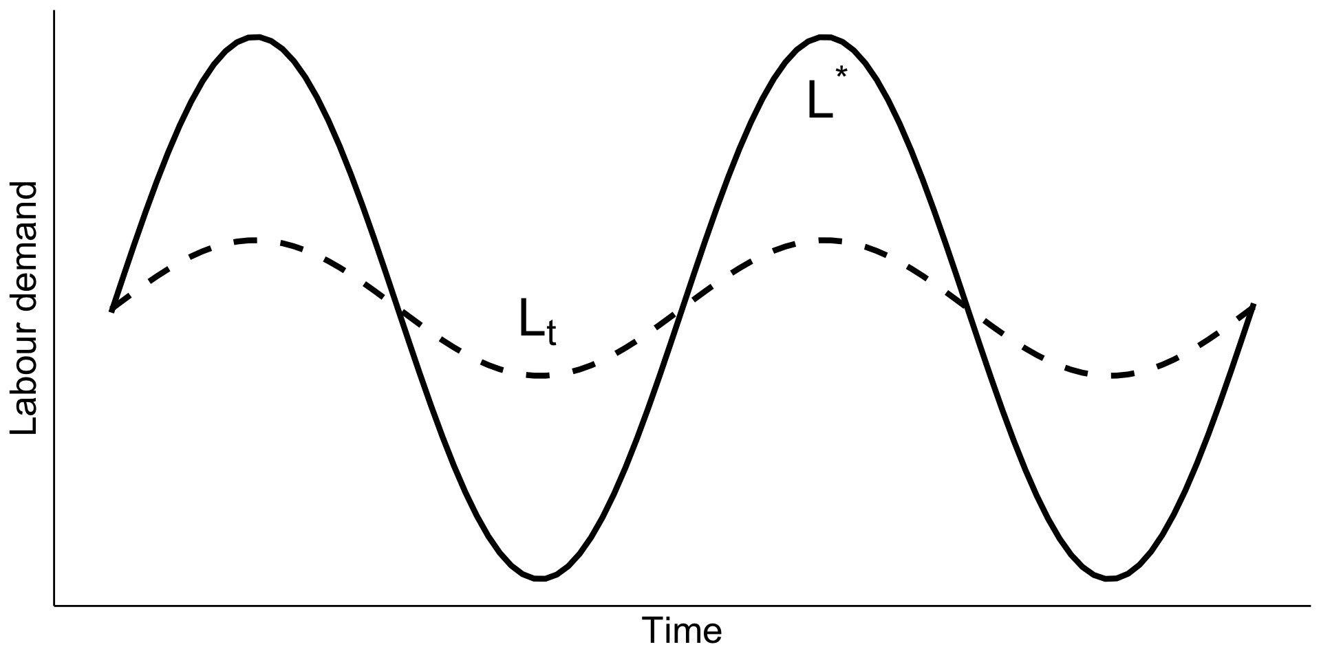
The theory was derived to analyse labour demand over the business cycle => $L^{\star }$ follows the business cycle

Highlight the smoothing!

• do not fire as much during recession because foresse hiring in the boom

• vice versa

BUT

• data suggests adjustments happen more quickly (maybe just means that $b$ smaller)

• symmetry forced by construction!

Dynamic model

Linear adjustment cost

$${\mathrm{\Pi }}_0={\int }_0^{\mathrm{\infty }}[F(L_t)-W_t{L}_t-C({\dot{L}}_t)]e^{-rt}dt$$

where $C\left({\dot{L}}_t\right)=\{\begin{array}{ll}{c}_h{\dot{L}}_t& \text{if }{\dot{L}}_t\ge 0\\ -c_f{\dot{L}}_t& \text{if }{\dot{L}}_t\le 0\end{array}$

Optimal labour demand path is derived from

$$\{\begin{array}{ll}{F}^{\prime }(L_t)=W_t+r{c}_h& \text{if }{\dot{L}}_t\ge 0\\ F^{\prime }(L_t)=W_t-r{c}_f& \text{if }{\dot{L}}_t<0\end{array}$$

• Nothing happens if $F^{\prime }(L_t)\in [W_t-r{c}_f,W_t+r{c}_h]$

• No smoothing: demand immediately jumps to stationary value if marginal productivities outweigh the costs

• Allows to analyse changes in hiring and firing costs separately

Dynamic model

Linear adjustment cost

Figure 9.10 Optimal employment over the cycle (Nickell 1986)

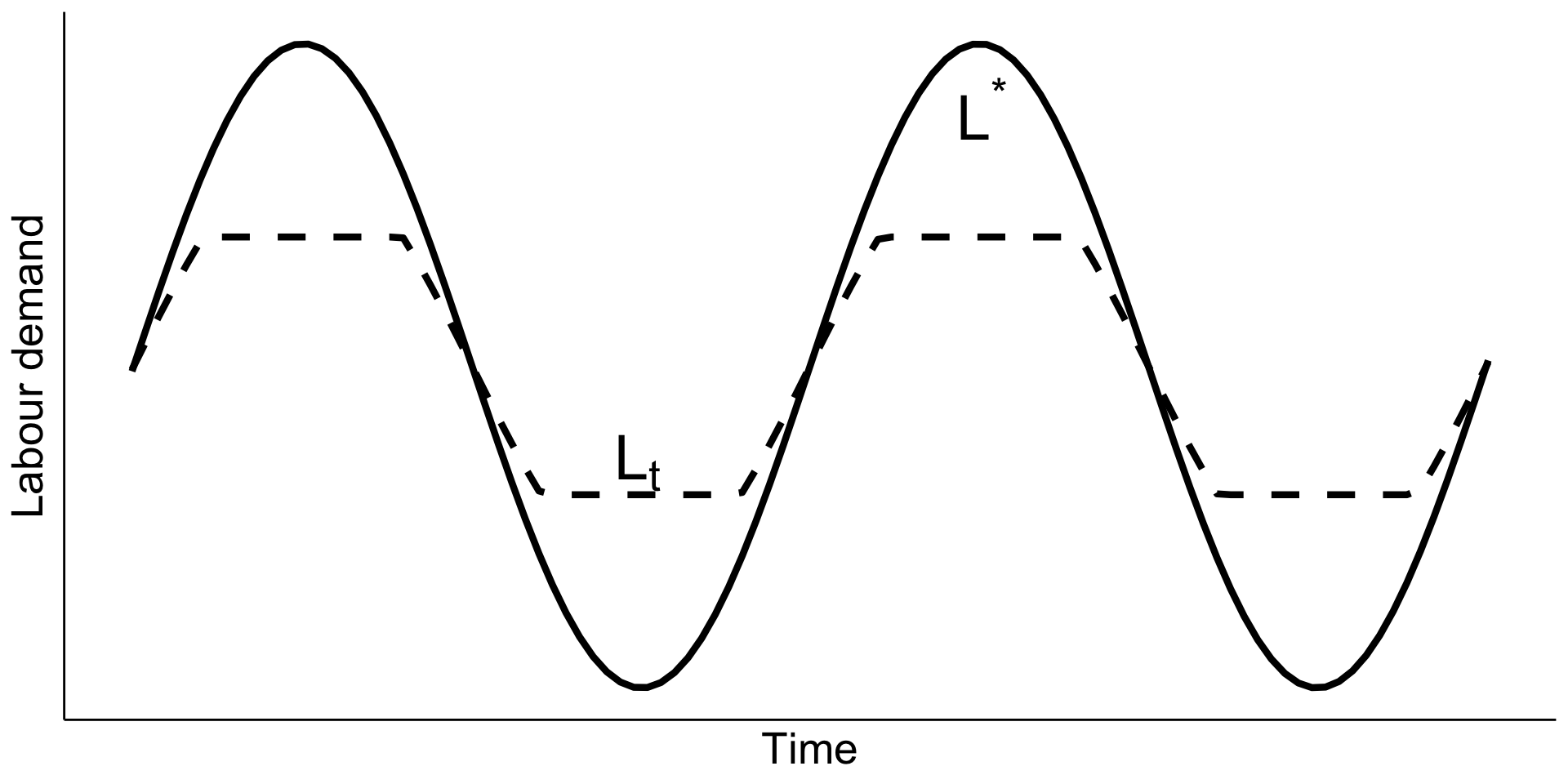
• There are two levels of optimal labour supply $L_h$ in the hiring phase and $L_f$ in the firing phase

• When things change, the firm immediately jumps to the new optimum if the deviation is large enough

• The levels $L_h$ and $L_f$ depend on the adjustment costs and need not be symmetric

Estimations of dynamic model

Empirical strategy for adjustment cost specification

Quadratic adjustment cost

• Assume linear quadratic production function

• Estimate $L_{it}=\lambda L_{i,t-1}+X_{it}\beta +{\mu }_i+{\epsilon }_{it}$

  • accounting for correlation between $L_{i,t-1}$ and ${\mu }_i+{\epsilon }_{it}$

Other adjustment costs and production functions

• Estimate Euler equation directly

• Current employment $L_t$ depends on past and future variables

• Appropriate econometric methods (Hamilton 1994 book)

• Mention uncertainty necessary to get estimable equation from models!

• Highlight the simple panel regression depends on functional assumptions for both $C$ and $F$!

Estimations of dynamic model

Some key results

• Adjustments happen fast (1-2 quarters) (Hamermesh 1996, chap. 7)

• Dynamic substitutes: utilization of capital increases with $L_t-L^{\ast }$

• Hours of work are adjusted faster than number of workers

  

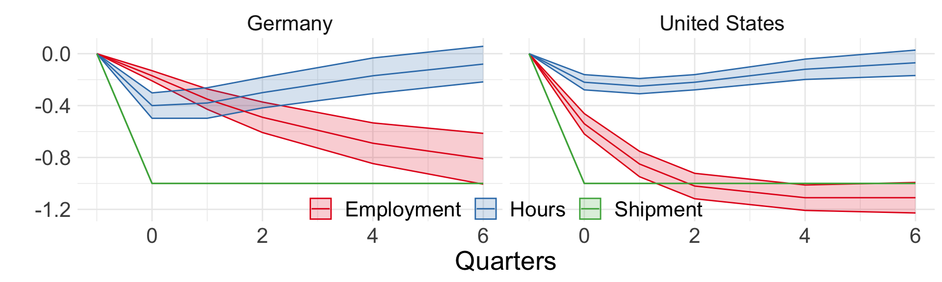
  Figure 1 from Houseman and Abraham (1993) (adjustment to demand shocks)

• Fewer estimates in the literature compared to static model

• mostly within 1 year, $\approx 50$% within 6 months

• adjustment costs are not quadratic (because fast) and not symmetric!

• Cahuc (2004) discusses: many US studies show $K$ and $L$ are dynamic substitutes

  • firms adjust $K$ faster when $L-L^{\star }$ is large

• The graph shows impulse responses following shock to shipments

  • short run:

    • Germany (with protections) adjusts hours before firing

    • US (without protections) nearly immediate firings

  • long run: both end up with fewer employees

Minimum wages and employment

Minimum wage and employment

What do the models we have considered so far predict?

• lower labour demand (both compensated and uncompensated)

• (maybe) higher labour supply

Any “problems” with these conclusions?

Typically not supported by empirical evidence!

• Only matters if $w_{min}>w^{\ast }$. This becomes strange with homogeneous labour.

• How employment is measured: number of workers or hours? Skills? Effort?

• Wage $\ne$ labour cost

Minimum wage and employment

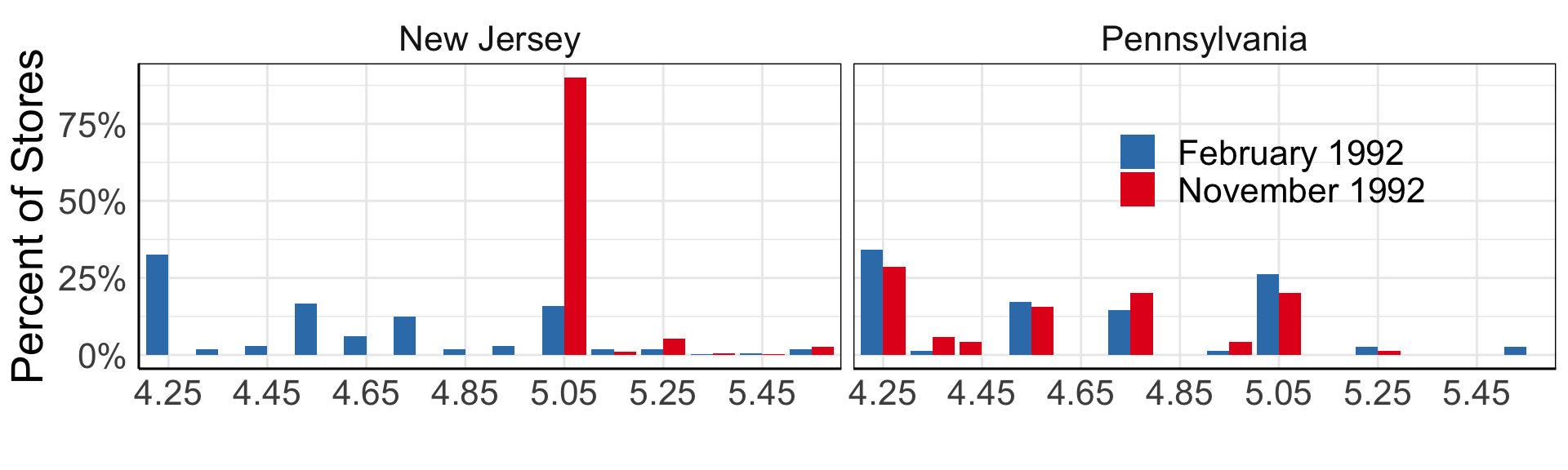
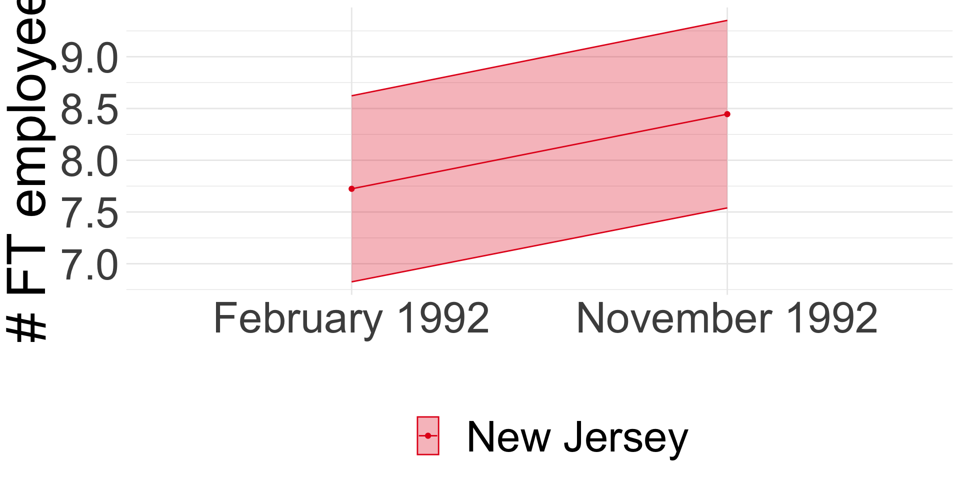
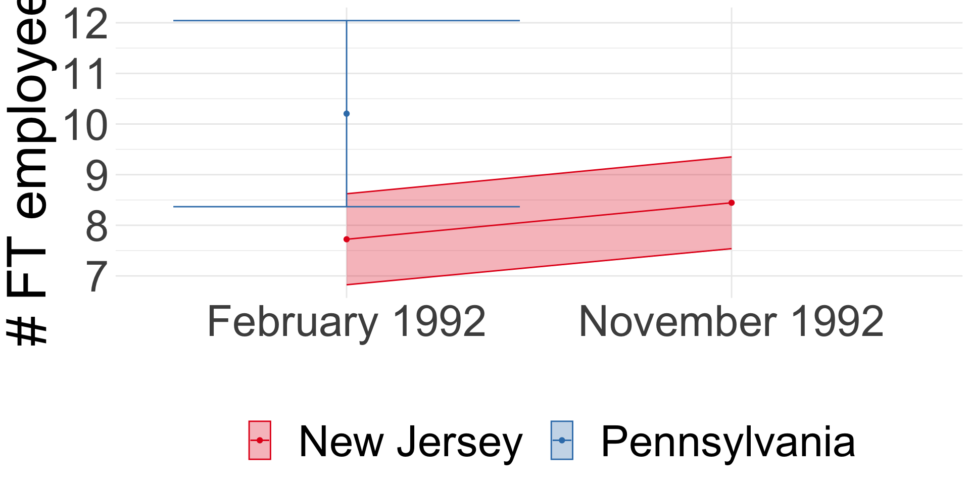
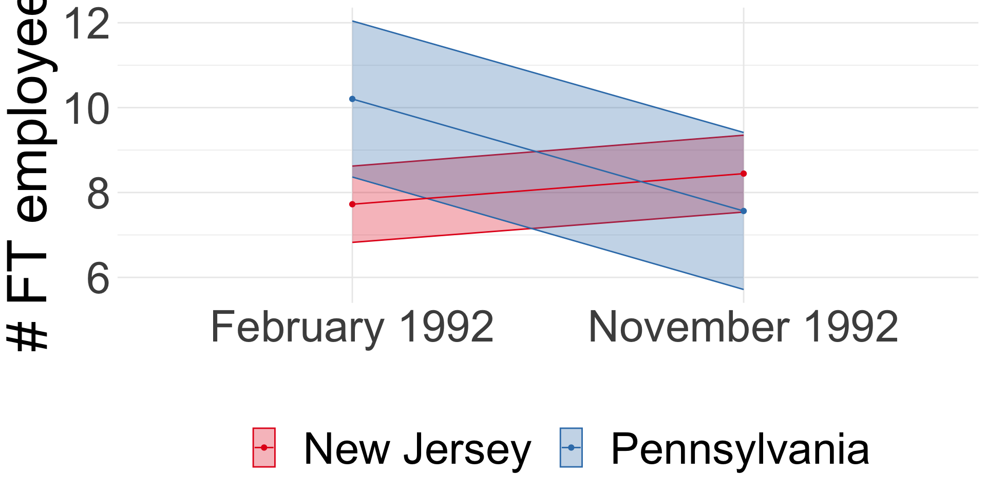
Card and Krueger (1994)

On April 1, 1992 minimum wage in New Jersey $\uparrow$ from $4.25 to $5.05.
It stayed at $4.25 in Pennsylvania.

Minimum wage and employment

Card and Krueger (1994): Difference-in-differences

1. Compare before and after:
   $E_{t1}^{NJ}-E_{t0}^{NJ}$ = 0.59 (se = 0.54)

Minimum wage and employment

Card and Krueger (1994): Difference-in-differences

1. Compare before and after:
   $E_{t1}^{NJ}-E_{t0}^{NJ}$ = 0.59 (se = 0.54)
2. Compare NJ and PA:
   $E_t^{NJ}-E_t^{PA}$ = -2.89 (se = 1.44)

Minimum wage and employment

Card and Krueger (1994): Difference-in-differences

1. Compare before and after:
   $E_{t1}^{NJ}-E_{t0}^{NJ}$ = 0.59 (se = 0.54)
2. Compare NJ and PA:
   $E_t^{NJ}-E_t^{PA}$ = -2.89 (se = 1.44)
3. Diff-in-diff:
   $(E_{t1}^{NJ}-E_{t0}^{NJ})-(E_{t1}^{PA}-E_{t0}^{PA})$ = 2.75 (se = 1.34)

STILL ongoing research field! next more recent paper with opposite conclusion

Minimum wage and employment

Jardim et al. (2022)

Seattle $\uparrow$ min wage from $9.47 up to

• $11 in April 2015
• $13 in January 2016

Causal design:

• synthetic control: weighted average of other counties that match pre-Seattle
• nearest neighbour matching: find “closest” worker outside of Seattle matching treated worker in Seattle

Minimum wage and employment

Jardim et al. (2022): synthetic control

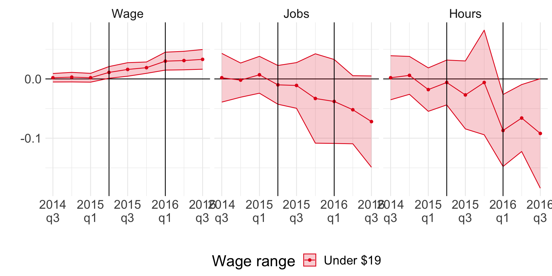
• Vertical lines show two episodes of min wage hikes

• Visible increase in observed wages

• Negative (but zero) effect on employment

• Negative effect on hours!

This is in the segment of the labour market affected by min wages.

What can we expect about results in other segments of the labour market?

Minimum wage and employment

Jardim et al. (2022): synthetic control

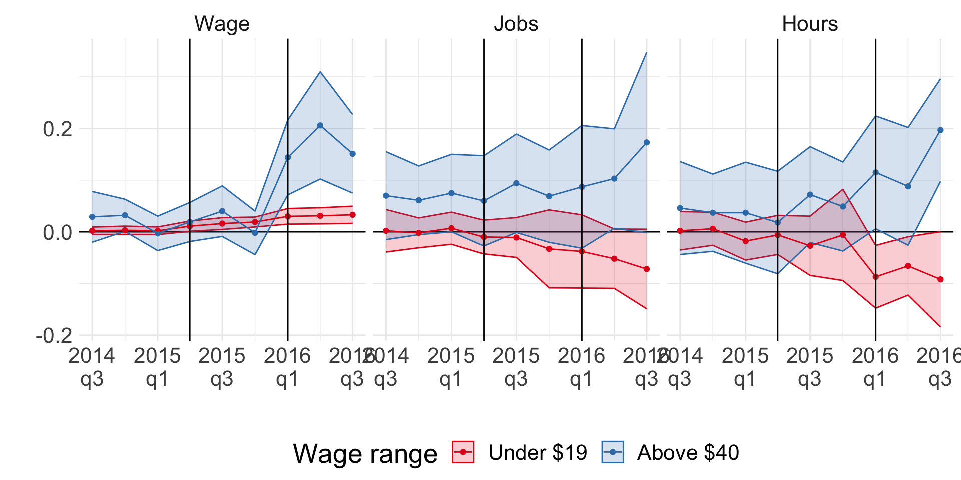
Discuss on next slide!

• Cascading effect on wages!

• Also positive effect on hours and employment!

• Probably general equilibrium at play?

Other issues:

• excluded employers with multiple locations that are believed to employ some 40 percent of Seattle’s low-wage earners.

• So, mom-and-pop retailers were counted, but McDonald’s franchises and the like were not!

• Some may argue that McDonald’s less elastic compared to mom-and-pop retailers => significant negative effects

Minimum wage and employment

Jardim et al. (2022): nearest neighbour matching

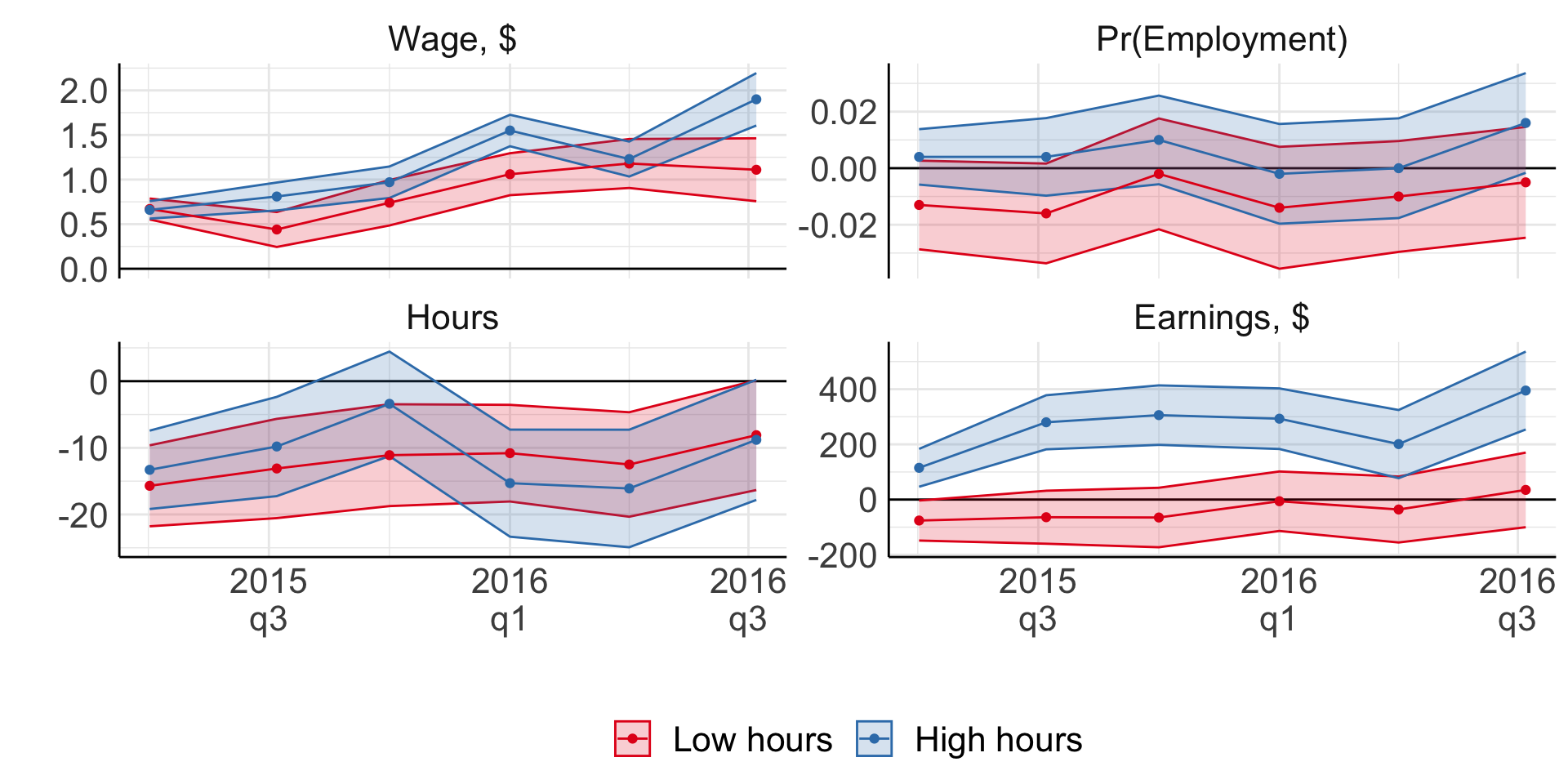
Minimum wage and employment

Jardim et al. (2022)

• Negative effect on hours worked stronger than on employment
• Experienced workers are better off

However,

• Potentially cascading effect
• Excluded large low-wage employers (like McDonald’s) (monopsony)

Reich, Allegretto, and Goddy (2017)

same policy + synthetic control = no change in employment

Short informal overview in https://anderson-review.ucla.edu/minimum-wage-primer-leamer/

Bridge to next slide:

Basic models say $L\downarrow$ when min wage $\uparrow$. What can explain opposite finding?

Minimum wage and employment

Monopsony

Source: Figure 3 from Brown (1999)

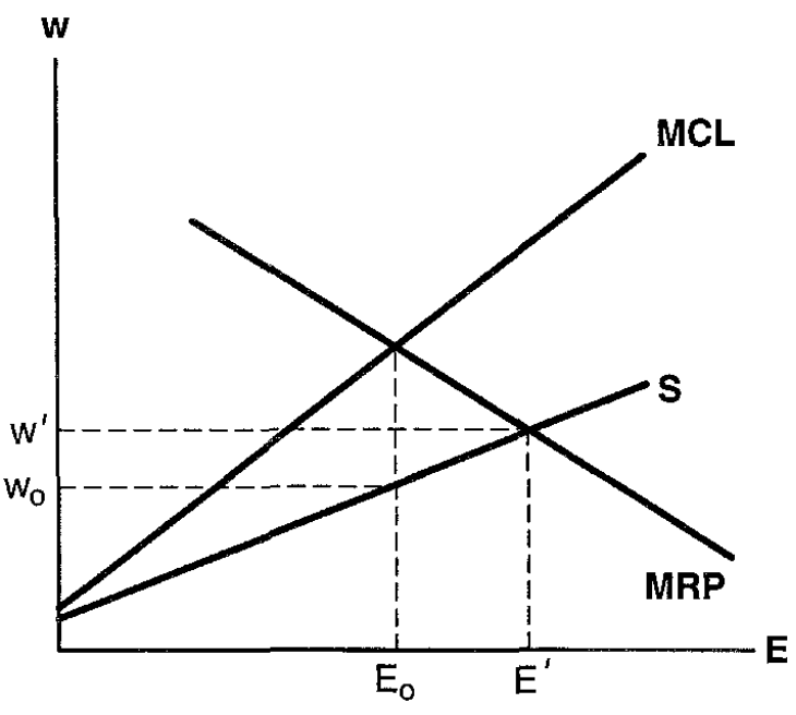
Another model: heterogeneous labour supply (skilled vs unskilled) see Cahuc (2004)

Alternative: basic models only have employment margin. In reality, many other margins for how firms might respond.

Minimum wage and other margins

Review in Clemens (2021)

• Price pass-through (Leung 2021; Renkin, Montialoux, and Siegenthaler 2022)
• Non-wage labour cost (Clemens, Kahn, and Meer 2018)
• Flexibility (theoretical Clemens and Strain 2020)
• Effort (Ku 2022; Coviello, Deserranno, and Persico 2022)
• Firm profit (Draca, Machin, and Van Reenen 2011; Bell and Machin 2018)
• Firm exit (Luca and Luca 2019; Dustmann et al. 2022)

Summary

• Basic static and dynamic models of labour demand

• Application to minimum wage policy

  • Ongoing research (little consensus)
  • Clear that basic models are insufficient
  • Typical frameworks: heterogeneous labour, monopsony
  • Non-wage margins important and can interact with labour supply

Next: Human Capital

References

Bell, Brian, and Stephen Machin. 2018. “Minimum Wages and Firm Value.” Journal of Labor Economics 36 (1): 159–95. https://doi.org/10.1086/693870.

Brown, Charles. 1999. “Chapter 32 Minimum Wages, Employment, and the Distribution of Income.” In Handbook of Labor Economics, 3:2101–63. Elsevier. https://doi.org/10.1016/S1573-4463(99)30018-3.

Cahuc, Pierre. 2004. Labor Economics. Cambridge (Mass.): MIT Press.

Card, David, and Alan B. Krueger. 1994. “Minimum Wages and Employment: A Case Study of the Fast-Food Industry in New Jersey and Pennsylvania.” The American Economic Review 84 (4): 772–93. https://www.jstor.org/stable/2118030.

Clemens, Jeffrey. 2021. “How Do Firms Respond to Minimum Wage Increases? Understanding the Relevance of Non-Employment Margins.” Journal of Economic Perspectives 35 (1): 51–72. https://doi.org/10.1257/jep.35.1.51.

Clemens, Jeffrey, Lisa B. Kahn, and Jonathan Meer. 2018. “The Minimum Wage, Fringe Benefits, and Worker Welfare.” NBER Working Paper. Working Paper Series. May 2018. https://doi.org/10.3386/w24635.

Clemens, Jeffrey, and Michael R. Strain. 2020. “Implications of Schedule Irregularity as a Minimum Wage Response Margin.” Applied Economics Letters 27 (20): 1691–94. https://doi.org/10.1080/13504851.2020.1713978.

Coviello, Decio, Erika Deserranno, and Nicola Persico. 2022. “Minimum Wage and Individual Worker Productivity: Evidence from a Large US Retailer.” Journal of Political Economy 130 (9): 2315–60. https://doi.org/10.1086/720397.

Draca, Mirko, Stephen Machin, and John Van Reenen. 2011. “Minimum Wages and Firm Profitability.” American Economic Journal: Applied Economics 3 (1): 129–51. https://doi.org/10.1257/app.3.1.129.

Dustmann, Christian, Attila Lindner, Uta Schönberg, Matthias Umkehrer, and Philipp vom Berge. 2022. “Reallocation Effects of the Minimum Wage*.” The Quarterly Journal of Economics 137 (1): 267–328. https://doi.org/10.1093/qje/qjab028.

Hamermesh, Daniel S. 1996. Labor Demand. Princeton University Press.

Houseman, Susan N, and Katharine G Abraham. 1993. “Labor Adjustment Under Different Institutional Structures: A Case Study of Germany and the United States.” NBER Working Paper 4548. Cambridge, MA. October 1993. https://www.nber.org/system/files/working_papers/w4548/w4548.pdf.

Jardim, Ekaterina, Mark C. Long, Robert Plotnick, Emma van Inwegen, Jacob Vigdor, and Hilary Wething. 2022. “Minimum-Wage Increases and Low-Wage Employment: Evidence from Seattle.” American Economic Journal: Economic Policy 14 (2): 263–314. https://doi.org/10.1257/pol.20180578.

Ku, Hyejin. 2022. “Does Minimum Wage Increase Labor Productivity? Evidence from Piece Rate Workers.” Journal of Labor Economics 40 (2): 325–59. https://doi.org/10.1086/716347.

Leung, Justin H. 2021. “Minimum Wage and Real Wage Inequality: Evidence from Pass-Through to Retail Prices.” The Review of Economics and Statistics 103 (4): 754–69. https://doi.org/10.1162/rest_a_00915.

Luca, Dara Lee, and Michael Luca. 2019. “Survival of the Fittest: The Impact of the Minimum Wage on Firm Exit.” NBER Working Paper. Working Paper Series. May 2019. https://doi.org/10.3386/w25806.

Nickell, S. J. 1986. “Chapter 9 Dynamic Models of Labour Demand.” In Handbook of Labor Economics, 1:473–522. Elsevier. https://doi.org/10.1016/S1573-4463(86)01012-X.

Reich, Michael, Sylvia Allegretto, and Anna Goddy. 2017. “Seattle’s Minimum Wage Experience 2015-16.” SSRN Electronic Journal. https://doi.org/10.2139/ssrn.3043388.

Renkin, Tobias, Claire Montialoux, and Michael Siegenthaler. 2022. “The Pass-Through of Minimum Wages into U.S. Retail Prices: Evidence from Supermarket Scanner Data.” The Review of Economics and Statistics 104 (5): 890–908. https://doi.org/10.1162/rest_a_00981.