2. Labour Supply

KAT.TAL.322 Advanced Course in Labour Economics

Labour supply

How people choose whether and how much they work?

Static model

Static labour supply

Model

• Utility from consumption of goods ($C$) and leisure ($L$): $U(C,L)$.
• Total time endowment $L_0$
• Agent chooses $h$ how much time to work such that $L=L_0-h$.
• Budget constraint is $C\le wh+Y\Rightarrow C+wL\le w{L}_0+Y$
  • $w$ is real hourly wage
  • $Y$ is non-labour income

$$\underset{C,h}{max}U(C,L_0-h)\text{subject to}C\le wh+Y$$

Static labour supply

Solution

First-order conditions of the Lagrangian are

$$U_C(C,L)=\lambda U_L(C,L)=\lambda w$$

Solution pair $C^{\ast }(w,Y)$ and $h^{\ast }(w,Y)$ satisfies

$$\frac{U_L(C^{\ast },L^{\ast })}{U_C(C^{\ast },L^{\ast })}=w\text{and}{C}^{\ast }=w{h}^{\ast }+Y$$

Static labour supply

Comparative statics

How does optimal labour supply change with $w$?

Marshallian (uncompensated) wage elasticity: ${\epsilon }_{hw}=\frac{\partial \ln h^{\ast }}{\partial \ln w}$

Hicksian (compensated) wage elasticity: ${\eta }_{hw}=\frac{\partial \ln \hat{h}}{\partial \ln w}$

Decomposition into substitution and income effects:

$${\epsilon }_{hw}={\eta }_{hw}+\frac{wh}{Y}{\epsilon }_{hY}$$

Static labour supply

Comparative statics

Source: Wikipedia

Static labour supply

Labour supply curve

Source: Wikipedia

Household model

Intrahousehold labour supply

Unitary model

Household represented by single utility function $U(C,L_1,L_2)$

Budget constraint $C+w_1{L}_1+w_2{L}_2\le Y_1+Y_2+(w_1+w_2)L_0$

• Simple extension of static model

• Not consistent with observed data

• In the non-earned part, only total income $Y_1+Y_2$ matters. T

• The solution doesn’t care about the distribution of these within household.

• Empirical works shows that it does matter. For example, paying children support to husband account or wife account.

Intrahousehold labour supply

Collective model

Individual utility functions $U_1(C_1,L_1),U_2(C_2,L_2)$

Budget constraint $C_1+C_2+w_1{L}_1+w_2{L}_2\le R_1+R_2+(w_1+w_2)L_0$

Partner utility constraint (Pareto efficiency) $U_2(C_2,L_2)\ge {\overline{U}}_2$

In this case, individual program can be represented by

$$\underset{C_i,L_i}{max}{U}_i(C_i,L_i)\text{s.t.}{C}_i+w_i{L}_i\le w_i{L}_0+{\mathrm{\Phi }}_i$$

where ${\mathrm{\Phi }}_i$ describes how resources $R_1+R_2$ are shared in the household.

For more, see (Cahuc 2004, chap. 1) and Chiappori (1992)

Intertemporal model

Intertemporal labour supply

Model

General utility function $U(C_0,\dots ,C_T;L_0,\dots ,L_T)$ (intractable)

Separable utility function $\sum _{t=0}^{T}U(C_t,L_t,t)$

Budget constraint $A_t=(1+r_t)A_{t-1}+B_t+w_t(1-L_t)-C_t$

• savings rate $r_t$
• total time normalized to one: $h_t+L_t=1$
• assets $A_t$
• non-labour income $B_t$

Intertemporal labour supply

Solution

$$\mathcal{L}=\sum _{t}U(C_t,L_t,t)-\sum _t{\nu }_t[A_t-(1+r_t)A_{t-1}-B_t-w_t(1-L_t)+C_t]$$

First-order conditions:

$$\begin{array}{rl}\frac{U_L(C_t,L_t,t)}{U_C(C_t,L_t,t)}=& w_t\\ {\nu }_t=& (1+r_{t+1}){\nu }_{t+1}\end{array}\mathrm{\forall }t\in [0,T]$$

Iterating over all periods: $\ln {\nu }_t=-\sum _{\tau =1}^t\ln (1+r_{\tau })+\ln {\nu }_0$

• MRS = w is maintained at every period BECAUSE we assumed intertemporal separability

• The optimal choice at every period depends on ${\mathbf{w}}_{\mathbf{t}}$ and ${\nu }_t$ (marginal utility of wealth)

• The term ${\nu }_t$ in turn depends both an age and overall potential ${\nu }_0$

• Initial value ${\nu }_0$ depends on all wages received during lifetime $\Rightarrow$ useful to disentangle temporary effects from permanent.

Intertemporal labour supply

Wage elasticities of labour supply

• Frisch elasticity ${\psi }_{hw}$ (holding ${\nu }_t$ constant)

• Marshallian elasticity ${\epsilon }_{hw}$ (takes into account ${\nu }_t$)

• Hicksian elasticity ${\eta }_{hw}$ (holding lifetime utility constant)

It is possible to show that ${\psi }_{hw}\ge {\eta }_{hw}\ge {\epsilon }_{hw}$

Interpretation

Transitory changes in wages affect labour supply more than permanent changes.

For derivations, see (Cahuc 2004, chap. 1 appendix 7.4)

Frisch elasticity: intertemporal substitution

Draw wage profile

Intertemporal labour supply

Example

Period utility $U(C_t,L_t,t)=\frac{C_t^{1+\rho }}{1+\rho }-{\beta }_t\frac{H_t^{1+\gamma }}{\gamma }$

FOC: $H_t^{\gamma }=\frac{1}{{\beta }_t}{\nu }_t{w}_t\Rightarrow \ln H_t=\frac{1}{\gamma }(-\ln {\beta }_t+\ln {\nu }_t+\ln w_t)$

1. Evolutionary changes along anticipated wage profile $\frac{\partial \ln H_t}{\partial \ln w_t}=\frac{1}{\gamma }>0$
2. Transitory changes $\frac{\partial \ln H_t}{\partial \ln w_t}=\frac{1}{\gamma }(1+\underset{<\approx 0}{\underbrace{\frac{\partial \ln {\nu }_0}{\partial \ln w_t}}})>0$
3. Permanent changes $\frac{\partial \ln H_t}{\partial \ln w_t}=\frac{1}{\gamma }(1+\frac{\partial \ln {\nu }_0}{\partial \ln w_t})\lessgtr 0$
4. Lottery win $\frac{\partial \ln H_t}{\partial \ln B_t}=\frac{1}{\gamma }\frac{\partial \ln {\nu }_0}{\partial \ln B_t}<0$

Estimations

Empirical specifications

Basic regression equation

$$\ln H_{it}={\alpha }_w\ln w_{it}+{\alpha }_R{\mathcal{R}}_{it}+\theta X_{it}+v_{it}$$

Interpretation of ${\alpha }_w$: Frisch, Marshallian or Hicksian? Depends on ${\mathcal{R}}_{it}$!

Empirical specifications

Two-stage budgeting

Solution method of lifecycle labour supply models (Blundell and Macurdy 1999)

1. Solve static labour supply model given $C_t={\mathcal{R}}_t+w_t{H}_t$
2. Solve for series ${\mathcal{R}}_1,\dots ,{\mathcal{R}}_T$ to maximize lifetime utility

$$\ln H_{it}={\alpha }_w\ln w_{it}+{\alpha }_R(C_{it}-w_{it}{H}_{it})+\theta X_{it}+v_{it}$$

Marshallian wage elasticity: ${\alpha }_w$

Income effect: ${\alpha }_{R}wH$

Hicksian wage elasticity: ${\alpha }_w-{\alpha }_{R}wH$

Empirical specifications

Frisch elasticity

Recall that $\ln {\nu }_t=-\sum _{\tau =1}^t\ln (1+r_{\tau })+\ln {\nu }_0\equiv -\ln (1+r)t+\ln {\nu }_0$ (if $r_{\tau }=r\mathrm{\forall }\tau$)

Substitute ${\alpha }_R{\mathcal{R}}_{it}=\rho t+{\alpha }_R\ln {\nu }_{0,i}$ into basic equation:

$$\begin{array}{rl}\ln H_{it}& =\rho t+{\alpha }_w\ln w_{it}+{\alpha }_R\ln {\nu }_{0,i}+\theta X_{it}+v_{it}\\ \mathrm{\Delta }\ln H_{it}& =\rho +{\alpha }_w\mathrm{\Delta }\ln w_{it}+\theta \mathrm{\Delta }{X}_{it}+\mathrm{\Delta }{v}_{it}\end{array}$$

Frisch wage elasticity: ${\alpha }_w$

Empirical specifications

Practical issues

• Wages and hours worked are endogeneous

• Hours ($H|H>0$) and participation ($H>0$)

• Measurement errors

• Measures of $C_{it}$

• Individual vs aggregate labour supply

Estimates

Observational data

Source: Pencavel (1986)

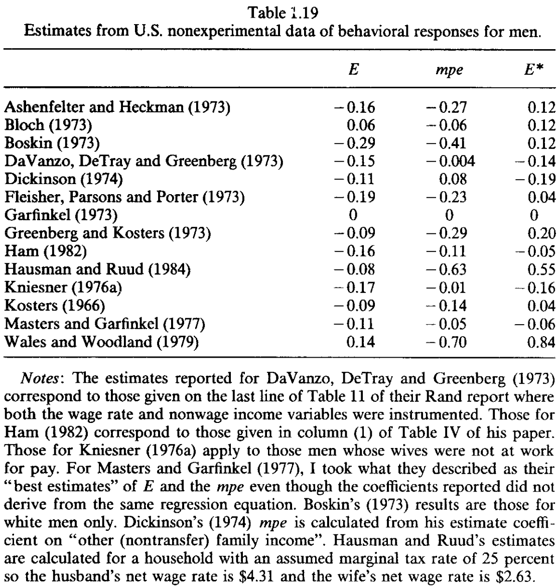
• Large variation between different estimates

• Some even report negative Hicksian elasticities!

• Most likely to do with endogeneity in the data => next experimental

Estimates

Experimental data: drop in tax rates in the UK 1978-92

Source: Blundell, Duncan, and Meghir (1998)

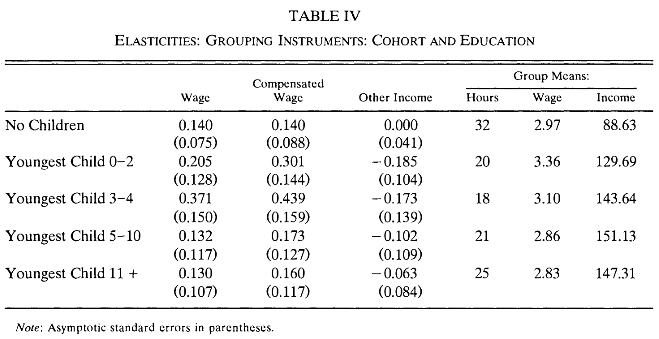
Now, Hicksian elasticities are of expected sign!

Are these values large? Some suggest participation is important, but overlooked in these studies!

Estimates

Intensive vs extensive margin

Source: Chetty et al. (2012)

Also some research on work effort for given hours of work (Dickinson 1999)

Micro vs macro

• Indivisible labour supply (Chetty et al. 2012)

• Optimization frictions (Chetty 2012)
  For example, hard to adjust hours continuously (contracts typically 8 hours); may be forced to search for another job.

Estimates

Measurement errors

Classical measurement error in $w_{it}$ attenuates the estimate of ${\alpha }_w$

“Denominator bias” $\downarrow {\alpha }_w$ if wages are computed as ratio of earning and hours with measurement errors. M. P. Keane (2011) computes average Hicksian elasticity

• among all papers: 0.31

• among papers with direct measure of $w_{it}$: 0.43

Estimates

Measurement of consumption

PSID (US) dataset only includes food consumption data

Consumption measure	Marshall	Hicks	Income	Frisch
PSID unadjusted	-0.442	0.094	-0.536	0.148
Food + imputed (food prices, demographics)	-0.468	0.328	-0.796	0.535
Food + imputed (house value, rent)	-0.313	0.220	-0.533	0.246

Source: (M. P. Keane 2011, Table 5)

Estimates

Micro vs macro elasticities

Macro elasticities of labour supply typically higher than micro estimates

M. Keane and Rogerson (2012) highlight:

• extensive vs intensive margin
• model misspecification due to human capital accumulation
• aggregation is not straightforward

Many ways to reconcile imply different mechanisms!

Estimates

Discrete choice dynamic programming

Incorporate discrete choices into model of labour supply

• labour force participation (Eckstein and Wolpin 1989)
• marriage (Van Der Klaauw 1996)
• fertility (Francesconi 2002)

M. P. Keane and Wolpin (2010) combine all + school and welfare participation choices

Uncompensated dynamic elasticity

Eckstein and Wolpin (1989)	5.0
Van Der Klaauw (1996)	3.6
Francesconi (2002)	5.6
M. P. Keane and Wolpin (2010)	2.8

Source: M. P. Keane (2011)

Summary

• Looked at standard models of labour supply

  • Important intertemporal considerations

• Mostly covered seminal papers, but many ongoing works

  • Tax and benefit policies
  • Cross-wage elasticities

Next: Labour Demand

References

Blundell, Richard, Alan Duncan, and Costas Meghir. 1998. “Estimating Labor Supply Responses Using Tax Reforms.” Econometrica 66 (4): 827–61. https://doi.org/10.2307/2999575.

Blundell, Richard, and Thomas Macurdy. 1999. “Chapter 27 - Labor Supply: A Review of Alternative Approaches.” In Handbook of Labor Economics, edited by Orley C. Ashenfelter and David Card, 3:1559–1695. Elsevier. https://doi.org/10.1016/S1573-4463(99)03008-4.

Cahuc, Pierre. 2004. Labor Economics. Cambridge (Mass.): MIT Press.

Chetty, Raj. 2012. “Bounds on Elasticities with Optimization Frictions: A Synthesis of Micro and Macro Evidence on Labor Supply.” Econometrica 80 (3): 969–1018. https://www.jstor.org/stable/41493842.

Chetty, Raj, Adam Guren, Day Manoli, and Andrea Weber. 2012. “Does Indivisible Labor Explain the Difference Between Micro and Macro Elasticities? A Meta-Analysis of Extensive Margin Elasticities.” NBER Macroeconomics Annual 27: 1–56. https://doi.org/10.1086/669170.

Chiappori, Pierre-André. 1992. “Collective Labor Supply and Welfare.” Journal of Political Economy 100 (3): 437–67. https://www.jstor.org/stable/2138727.

Dickinson, David L. 1999. “An Experimental Examination of Labor Supply and Work Intensities.” Journal of Labor Economics 17 (4): 638–70. https://doi.org/10.1086/209934.

Eckstein, Zvi, and Kenneth I. Wolpin. 1989. “Dynamic Labour Force Participation of Married Women and Endogenous Work Experience.” The Review of Economic Studies 56 (3): 375–90. https://doi.org/10.2307/2297553.

Francesconi, Marco. 2002. “A Joint Dynamic Model of Fertility and Work of Married Women.” Journal of Labor Economics 20 (2): 336–80. https://doi.org/10.1086/338220.

Keane, Michael P. 2011. “Labor Supply and Taxes: A Survey.” Journal of Economic Literature 49 (4): 961–1075. https://doi.org/10.1257/jel.49.4.961.

Keane, Michael P., and Kenneth I. Wolpin. 2010. “The Role of Labor and Marriage Markets, Preference Heterogeneity, and the Welfare System in the Life Cycle Decisions of Black, Hispanic, and White Women.” International Economic Review 51 (3): 851–92. https://www.jstor.org/stable/40784808.

Keane, Michael, and Richard Rogerson. 2012. “Micro and Macro Labor Supply Elasticities: A Reassessment of Conventional Wisdom.” Journal of Economic Literature 50 (2): 464–76. https://doi.org/10.1257/jel.50.2.464.

Pencavel, John. 1986. “Chapter 1 Labor Supply of Men: A Survey.” In Handbook of Labor Economics, 1:3–102. Elsevier. https://doi.org/10.1016/S1573-4463(86)01004-0.

Van Der Klaauw, Wilbert. 1996. “Female Labour Supply and Marital Status Decisions: A Life-Cycle Model.” The Review of Economic Studies 63 (2): 199–235. https://doi.org/10.2307/2297850.