Intelligence and Income

Authors

Affiliations

Nurfatima Jandarova

Aldo Rustichini

Center of Excellence in Tax Systems Research, Tampere University

Department of Economics, University of Minnesota

Introduction

• Cognitive and noncognitive skills and family background are important determinants of education

• Policies can change the relative importance of these factors (Ichino, Rustichini, and Zanella 2022)

• Growing evidence on interplay between genes and environment (Rustichini et al. 2023)

Contributions

Determinants of education: Heckman, Stixrud, and Urzua (2006), Almlund et al. (2011), Björklund and Salvanes (2011), Ichino, Rustichini, and Zanella (2022)

Genes and environment in education: Rustichini et al. (2023)

UK Household Longitudinal Study (2009-)

Working sample: 22 881 individuals

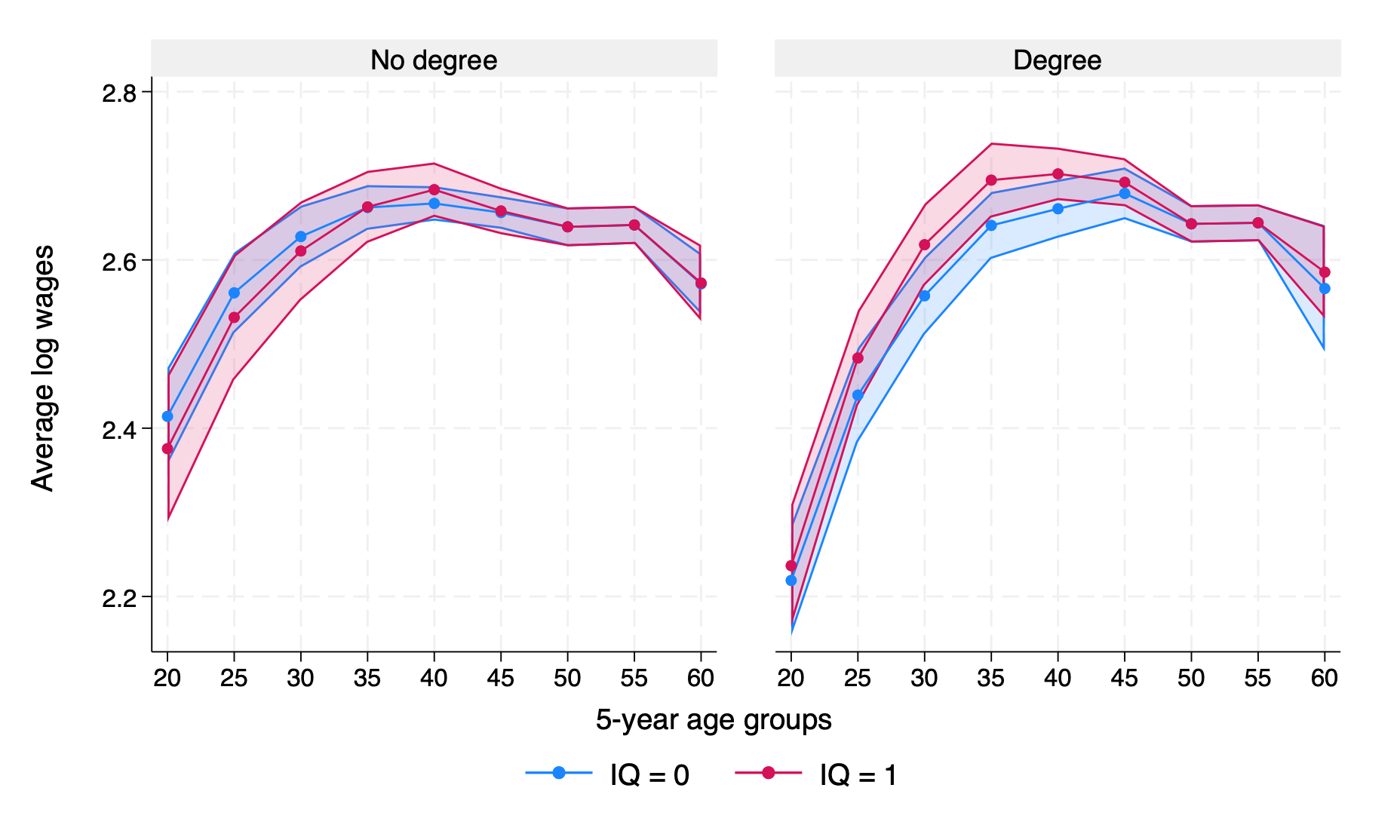
• college: ever had HE degree as highest qualification

• predicted discounted present value of earnings

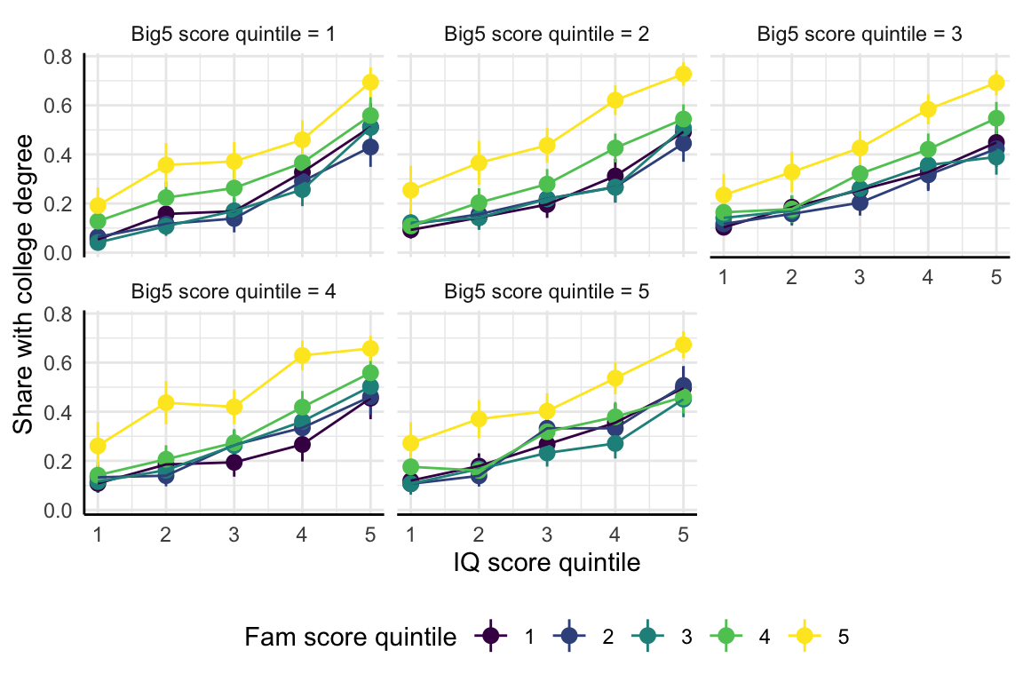
• cognitive test scores , Big 5 personality scores

• parental background: education and employment status

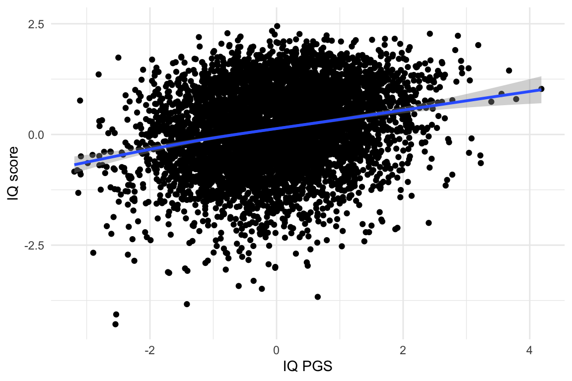
METADAC

Genotyped subsample: 3 413 individuals

• polygenic score (PGS) of fluid intelligence (Savage et al. 2018)

College and individual characteristics

df %>% 
  as_survey_design(ids = c_psu, 
                   strata = c_strata, 
                   weights = c_indinub_xw) %>% 
  group_by(gscorep_qnt, etap_fam_qnt, etap_big5_qnt) %>% 
  summarise(cmean = survey_mean(college, vartype = 'ci')) %>% 
  ggplot(aes(x = gscorep_qnt, 
             y = cmean, ymin = cmean_low, ymax = cmean_upp, 
             colour = factor(etap_fam_qnt), 
             group = factor(etap_fam_qnt))) + 
  geom_pointrange() + 
  geom_line() + 
  facet_wrap(~ etap_big5_qnt, scales = 'fixed', 
             labeller = as_labeller(function(x) 
               paste('Big5 score quintile =', x))) + 
  labs(x = 'IQ score quintile', y = 'Share with college degree', 
       colour = 'Fam score quintile') + 
  scale_colour_viridis_d() + 
  theme_minimal() + 
  theme(legend.position = 'bottom', 
        axis.line = element_line())

Probability of college

tab1 <- read_dta('tab1.dta')
tab1 <- tab1 %>% rename(std.error = std_err)
tab1 <- tab1 %>% 
  mutate(p.value = pnorm(abs(estimate) / std.error, 
                         lower.tail = FALSE))

tab1_list <- tab1 %>% 
  nest(.by = c(cohort, spec)) %>% 
  mutate(cohort = str_extract(cohort, '(?<=19)[:digit:]{2}')) %>% 
  unite('id', spec, cohort, sep = '') %>% 
  deframe()

tab1_ols50 <- list(tidy = tab1_list$ols50,
                   glance = tab1_list$ols50 %>% distinct(N))
tab1_lme50 <- list(tidy = tab1_list$logme50, 
                   glance = tab1_list$logme50 %>% distinct(N))
tab1_ols65 <- list(tidy = tab1_list$ols65,
                   glance = tab1_list$ols65 %>% distinct(N))
tab1_lme65 <- list(tidy = tab1_list$ols65,
                   glance = tab1_list$ols65 %>% distinct(N))
tab1_ols80 <- list(tidy = tab1_list$ols80,
                   glance = tab1_list$ols80 %>% distinct(N))
tab1_lme80 <- list(tidy = tab1_list$ols80,
                   glance = tab1_list$ols80 %>% distinct(N))

class(tab1_ols50) <- 'modelsummary_list'
class(tab1_lme50) <- 'modelsummary_list'
class(tab1_ols65) <- 'modelsummary_list'
class(tab1_lme65) <- 'modelsummary_list'
class(tab1_ols80) <- 'modelsummary_list'
class(tab1_lme80) <- 'modelsummary_list'

modelsummary(list(OLS = tab1_ols50, 
                  'Logit ME' = tab1_lme50, 
                  OLS = tab1_ols65, 
                  'Logit ME' = tab1_lme65, 
                  OLS = tab1_ols80, 
                  'Logit ME' = tab1_lme80), 
             coef_map = c(g_score_std = 'IQ score', 
                          eta_fam_score_std = 'Fam score', 
                          eta_big5_score_std = 'Big5 score'), 
             gof_map = list(list(raw = 'N', clean = 'Obs.', 
                                 fmt = function(x) format(x, 
                                                          big.mark = ' '))), 
             stars = c('*' = .05, '**' = .01, '***' = 0.001)) %>% 
  group_tt(j = list('Born in 1950-64' = 2:3, 
                    'Born in 1965-79' = 4:5, 
                    'Born in 1980-94' = 6:7))

	Born in 1950-64		Born in 1965-79		Born in 1980-94
	OLS	Logit ME	OLS	Logit ME	OLS	Logit ME
* p < 0.05, ** p < 0.01, *** p < 0.001
IQ score	0.137***	0.152***	0.151***	0.151***	0.130***	0.130***
	(0.005)	(0.007)	(0.005)	(0.005)	(0.006)	(0.006)
Fam score	0.050***	0.054***	0.077***	0.077***	0.074***	0.074***
	(0.005)	(0.008)	(0.006)	(0.006)	(0.006)	(0.006)
Big5 score	0.006	0.015**	0.010*	0.010*	0.014*	0.014*
	(0.006)	(0.006)	(0.006)	(0.006)	(0.006)	(0.006)
Obs.	9 539	9 539	10 586	10 586	8 409	8 409

SEM of college and wages

tab3 <- read_dta('tab3.dta')
tab3 <- tab3 %>% rename(std.error = std_err)
tab3 <- tab3 %>% 
  mutate(p.value = pnorm(abs(estimate) / std.error, 
                         lower.tail = FALSE))

tab3_list <- tab3 %>% 
  nest(.by = c(cohort, depvar)) %>% 
  mutate(cohort = str_extract(cohort, '(?<=19)[:digit:]{2}')) %>% 
  unite('id', depvar, cohort, sep = '') %>% 
  deframe()

tab3_wage4550 <- list(tidy = tab3_list$wage4550,
                   glance = tab3_list$wage4550 %>% distinct(N))
tab3_college50 <- list(tidy = tab3_list$college50, 
                   glance = tab3_list$college50 %>% distinct(N))
tab3_wage4565 <- list(tidy = tab3_list$wage4565,
                   glance = tab3_list$wage4565 %>% distinct(N))
tab3_college65 <- list(tidy = tab3_list$college65,
                   glance = tab3_list$college65 %>% distinct(N))
tab3_wage4580 <- list(tidy = tab3_list$wage4580,
                   glance = tab3_list$wage4580 %>% distinct(N))
tab3_college80 <- list(tidy = tab3_list$college80,
                   glance = tab3_list$college80 %>% distinct(N))

class(tab3_wage4550) <- 'modelsummary_list'
class(tab3_college50) <- 'modelsummary_list'
class(tab3_wage4565) <- 'modelsummary_list'
class(tab3_college65) <- 'modelsummary_list'
class(tab3_wage4580) <- 'modelsummary_list'
class(tab3_college80) <- 'modelsummary_list'

modelsummary(list('Pred. wage' = tab3_wage4550, 
                  'College' = tab3_college50, 
                  'Pred. wage' = tab3_wage4565, 
                  'College' = tab3_college65, 
                  'Pred. wage' = tab3_wage4580, 
                  'College' = tab3_college80), 
             coef_map = c(college = 'College',  
                          g_score_std = 'IQ score', 
                          eta_fam_score_std = 'Fam score', 
                          eta_big5_score_std = 'Big5 score', 
                          indirect = 'Indirect effect', 
                          total = 'Total effect'), 
             gof_map = list(list(raw = 'N', clean = 'Obs.', 
                                 fmt = function(x) format(x, 
                                                          big.mark = ' '))), 
             stars = c('*' = .05, '**' = .01, '***' = 0.001)) %>% 
  group_tt(j = list('Born in 1950-64' = 2:3, 
                    'Born in 1965-79' = 4:5, 
                    'Born in 1980-94' = 6:7)) %>% 
  style_tt(i = -1:13, fontsize = 0.75, 
           tabularray_inner = "rowsep = {-.22em}, colsep = {.4em}") %>% 
  style_tt(i = 8, line = 'b', line_width = .001)

	Born in 1950-64		Born in 1965-79		Born in 1980-94
	Pred. wage	College	Pred. wage	College	Pred. wage	College
* p < 0.05, ** p < 0.01, *** p < 0.001
College	0.820***		0.804***		0.651***
	(0.020)		(0.016)		(0.015)
IQ score	0.082***	1.018***	0.077***	0.917***	0.045***	0.788***
	(0.009)	(0.046)	(0.007)	(0.039)	(0.007)	(0.044)
Fam score		0.382***		0.492***		0.453***
		(0.051)		(0.040)		(0.041)
Big5 score		0.082*		0.081**		0.128***
		(0.037)		(0.033)		(0.037)
Indirect effect	0.126***		0.136***		0.096***
	(0.006)		(0.005)		(0.005)
Total effect	0.208***		0.213***		0.140***
	(0.009)		(0.007)		(0.007)
Obs.	9 496	9 496	10 488	10 488	8 382	8 382

  # kable_styling(font_size = 8) %>% 
  # row_spec(8, hline_after = TRUE) %>% 
  # add_header_above(c(' ' = 1, 
  #                    'Born in 1950-64' = 2, 
  #                    'Born in 1965-79' = 2, 
  #                    'Born in 1980-94' = 2))

Model

Individuals described by $z\in Z=\mathrm{\Theta }\times X\times Y$

• intelligence $\theta \in \mathrm{\Theta }$
• family advantage score $x\in X$
• Big 5 personality score $y\in Y$

Human capital $H\equiv \{nc,c\}$ (no college vs college)

DPV of earnings $W(h,z,\delta )=\sum _{a=18}^{65}{\delta }^{a-18}W(h,z,a)$

Choose effort $e\in {\mathbb{R}}_{+}$ to acquire human capital $h=c$ given cost $\frac{c(e)}{\mathrm{\Gamma }(z)}$

$$\underset{e}{max}\pi (e)[W(c,z,\delta )-W(nc,z,\delta )]-\frac{c(e)}{\mathrm{\Gamma }(z)}$$

Solution

Denote $A=(W(c,z,\delta )-W(nc,z,\delta ))\mathrm{\Gamma }(z)$. Then, optimal effort solution

$$E^{\star }(A;\pi )\equiv \arg \underset{e}{max}\pi (e)A-e$$

$\mathrm{\Pi }$ is the set of functions $\pi :{\mathbb{R}}_{+}\to [0,1]$ that are strictly increasing, concave, continuous at 0, $\pi (0)=0$, $\underset{x\to \mathrm{\infty }}{lim}\pi (x)=1$.

For $P(A)$ increasing in $A$ and upper semi-continuous in $\mathrm{\Delta }W$, $\mathrm{\exists }\pi \in \mathrm{\Pi }$ such that

$$P(A)=\pi (E^{\star }(A;\pi ))$$

Estimation

We consider four functional forms that can describe $P(A)$:

• Linear probability model $P(A)=A$
• Logit $P(A)=(1+e^{-A}{)}^{-1}$
• Logit power $P(A)=(1+e^{-A}{)}^{-\kappa },\kappa \in {\mathbb{R}}_{+}$
• Cutoff power $P(A)=min\{max\{A,0{\}}^{\kappa },1\},\kappa \in {\mathbb{R}}_{+}$

Two-step estimation:

1. Given $\delta$ and $\kappa$, fit $P(A)$ to the observed college indicators.
2. Grid search $\hat{\delta }$ and $\hat{\kappa }$ that minimise sum of squared residuals.

Results

tab4 <- read_dta('tab4.dta')
tab4 <- tab4 %>% rename(std.error = std_error)
tab4 <- tab4 %>% 
  mutate(print_error = if_else(is.na(boot_error), 
                               std.error, boot_error))
tab4 <- tab4 %>% 
  mutate(p.value = pnorm(abs(estimate) / print_error, 
                         lower.tail = FALSE))

tab4_list <- tab4 %>% nest(.by = c(spec)) %>% deframe()

tab4_lpm <- list(tidy = tab4_list$LPM,
                 glance = tab4_list$LPM %>% 
                   distinct(rmse, mean_cp, sd_cp, 
                            delta, power, N))
tab4_log <- list(tidy = tab4_list$Logit, 
                 glance = tab4_list$Logit %>% 
                   distinct(rmse, mean_cp, sd_cp, 
                            delta, power, N))
tab4_logp <- list(tidy = tab4_list$`Logit power`, 
                  glance = tab4_list$`Logit power` %>% 
                    distinct(rmse, mean_cp, sd_cp, 
                             delta, power, N))
tab4_cutp <- list(tidy = tab4_list$`Cutoff power`, 
                  glance = tab4_list$`Cutoff power` %>% 
                    distinct(rmse, mean_cp, sd_cp, 
                             delta, power, N))

class(tab4_lpm) <- 'modelsummary_list' 
class(tab4_log) <- 'modelsummary_list'
class(tab4_logp) <- 'modelsummary_list'
class(tab4_cutp) <- 'modelsummary_list'

gof_tab <- list(list(raw = 'N', 
                     clean = 'Obs.', 
                     fmt = function(x) format(x, big.mark = ' ')), 
                list(raw = 'delta', 
                     clean = '$\\delta$', 
                     fmt = 3), 
                list(raw = 'power', 
                     clean = '$\\kappa$', 
                     fmt = 2), 
                list(raw = 'mean_cp', 
                     clean = 'College premium mean', 
                     fmt = 2), 
                list(raw = 'sd_cp', 
                     clean = 'College premium sd', 
                     fmt = 2))
modelsummary(list('LPM' = tab4_lpm, 
                  'Logit' = tab4_log, 
                  'Logit power\\footnotemark[1]' = tab4_logp, 
                  'Cutoff power\\footnotemark[1]' = tab4_cutp), 
             statistic = '({print_error})', 
             coef_map = c(g_score_std = 'IQ score', 
                          eta_fam_score_std = 'Fam score', 
                          eta_big5_score_std = 'Big5 score', 
                          sdd_earn_2 = 'College premium, std'), 
             gof_map = gof_tab, 
             stars = c('*' = .05, '**' = .01, '***' = 0.001), 
             width = c(0.27, rep((1 - 0.25) / 4, 4)), 
             escape = FALSE, notes = list(`1`= 'Bootstrapped standard errors')) %>% 
  style_tt(i = 0:15, fontsize = 0.8, 
           tabularray_inner = "rowsep={-.22em}, colsep = {.4em}")

	LPM	Logit	Logit power\footnotemark[1]	Cutoff power\footnotemark[1]
* p < 0.05, ** p < 0.01, *** p < 0.001
1 Bootstrapped standard errors
IQ score	0.118***	0.089***	0.104***	0.108***
	(0.005)	(0.007)	(0.006)	(0.006)
Fam score	0.061***	0.054***	0.058***	0.058***
	(0.004)	(0.004)	(0.004)	(0.004)
Big5 score	0.025***	0.038***	0.032***	0.031***
	(0.003)	(0.004)	(0.004)	(0.004)
College premium, std	0.026***	0.060***	0.042***	0.040***
	(0.006)	(0.009)	(0.007)	(0.007)
Obs.	31 571	31 571	31 571	31 571
$\delta$	0.925	0.925	0.925	0.925
$\kappa$			2.90	1.20
College premium mean	36.95	36.95	36.95	36.95
College premium sd	9.77	9.77	9.77	9.77

Results with polygenic scores

Simple logit without college premium

tab6a <- read_dta('tab6a.dta')
tab6a <- tab6a %>% rename(std.error = std_error)
tab6a <- tab6a %>% 
  mutate(p.value = pnorm(abs(estimate) / std.error, 
                         lower.tail = FALSE))
tab6a_list <- tab6a %>% nest(.by = c(spec)) %>% deframe()

tab6a_lpm <- list(tidy = tab6a_list$LPM,
                  glance = tab6a_list$LPM %>% distinct(N))
tab6a_log <- list(tidy = tab6a_list$`Logit ME`, 
                  glance = tab6a_list$`Logit ME` %>% distinct(N))

class(tab6a_lpm) <- 'modelsummary_list'
class(tab6a_log) <- 'modelsummary_list'

gof_tab <- list(list(raw = 'N', 
                     clean = 'Obs.', 
                     fmt = function(x) format(x, big.mark = ' ')))
modelsummary(list('LPM' = tab6a_lpm, 
                  'Logit ME' = tab6a_log), 
             coef_map = c(pgs_std_cobs_hm3p = 'IQ PGS', 
                          eta_fam_score_std = 'Fam score', 
                          eta_big5_score_std = 'Big5 score'), 
             gof_map = gof_tab, 
             stars = c('*' = .05, '**' = .01, '***' = 0.001), 
             width = 1)

	LPM	Logit ME
* p < 0.05, ** p < 0.01, *** p < 0.001
IQ PGS	0.067***	0.066***
	(0.007)	(0.007)
Fam score	0.094***	0.118***
	(0.008)	(0.010)
Big5 score	0.019**	0.019**
	(0.008)	(0.008)
Obs.	3 602	3 602

Results with polygenic scores

tab6 <- read_dta('tab6.dta')
tab6 <- tab6 %>% rename(std.error = std_error)
tab6 <- tab6 %>% 
  mutate(p.value = pnorm(abs(estimate) / std.error, 
                         lower.tail = FALSE))
tab6_list <- tab6 %>% nest(.by = c(spec)) %>% deframe()

tab6_lpm <- list(tidy = tab6_list$LPM,
                 glance = tab6_list$LPM %>% 
                   distinct(mean_cp, sd_cp, delta, power, N))
tab6_log <- list(tidy = tab6_list$Logit, 
                 glance = tab6_list$Logit %>% 
                   distinct(mean_cp, sd_cp, delta, power, N))
tab6_logp <- list(tidy = tab6_list$`Logit power`, 
                  glance = tab6_list$`Logit power` %>% 
                    distinct(mean_cp, sd_cp, delta, power, N))
tab6_cutp <- list(tidy = tab6_list$`Cutoff power`, 
                  glance = tab6_list$`Cutoff power` %>% 
                    distinct(mean_cp, sd_cp, delta, power, N))

class(tab6_lpm) <- 'modelsummary_list'
class(tab6_log) <- 'modelsummary_list'
class(tab6_logp) <- 'modelsummary_list'
class(tab6_cutp) <- 'modelsummary_list'

gof_tab <- list(list(raw = 'N', 
                     clean = 'Obs.', 
                     fmt = function(x) format(x, big.mark = ' ')), 
                list(raw = 'delta', 
                     clean = '$\\delta$', 
                     fmt = 3), 
                list(raw = 'power', 
                     clean = '$\\kappa$', 
                     fmt = 2), 
                list(raw = 'mean_cp', 
                     clean = 'College premium mean', 
                     fmt = 2), 
                list(raw = 'sd_cp', 
                     clean = 'College premium sd', 
                     fmt = 2))
modelsummary(list('LPM' = tab6_lpm, 
                  'Logit' = tab6_log, 
                  'Logit power' = tab6_logp, 
                  'Cutoff power' = tab6_cutp), 
             coef_map = c(pgsp_cobs_hm3p = 'IQ PGS', 
                          etap_fam = 'Fam score', 
                          etap_big5 = 'Big5 score', 
                          diff4_earn = 'College premium, std'), 
             gof_map = gof_tab, 
             stars = c('*' = .05, '**' = .01, '***' = 0.001), 
             escape = FALSE, 
             width = c(0.27, rep((1 - 0.27) / 4, 4))) %>% 
  style_tt(i = 0:14, fontsize = .9, 
           tabularray_inner = "rowsep={-.2em}, colsep = {.3em}")

	LPM	Logit	Logit power	Cutoff power
* p < 0.05, ** p < 0.01, *** p < 0.001
IQ PGS	0.038***	0.034**	0.036**	0.037***
	(0.011)	(0.012)	(0.012)	(0.011)
Fam score	0.085***	0.154***	0.146***	0.134***
	(0.008)	(0.011)	(0.011)	(0.010)
Big5 score	0.109***	0.102**	0.105**	0.115***
	(0.031)	(0.034)	(0.034)	(0.034)
College premium, std	0.007**	0.006**	0.006**	0.007**
	(0.002)	(0.002)	(0.002)	(0.002)
Obs.	3 602	3 602	3 602	3 602
$\delta$	0.925	0.925	0.925	0.925
$\kappa$			2.90	1.20
College premium mean	84.86	84.86	84.86	84.86
College premium sd	14.27	14.27	14.27	14.27

Summary

• Revisit role of intelligence, personality and family characteristics in education choice

• Conditions linking econometric specification to individual optimization

• Further analysis with polygenic scores

Appendices

Predicted wage profile

Intelligence score

Combine individual test scores using confirmatory factor analysis

Using "tree" as default layout

Big 5 personality score

Combine individual test scores using principal component analysis

Score	Loading
Agreeableness	0.4408
Conscientiousness	0.4970
Extraversion	0.4628
Neuroticism	-0.3751
Openness	0.4514

PC1 explains 36% of variation in the data

Family advantage score

Combine education of parents and their employment status using principal component analysis

Variable	Loading (mother)	Loading (father)
Years of education	0.4020	0.4286
Work	0.2243	0.5527
Dead	-0.0889	-0.2958
Absent	-0.2042	-0.4023

PC1 explains 23% of variation in the data

METADAC vs full sample

bal <- read_dta('tab-bal.dta') 
bal_list <- bal %>% nest(.by = dataset) %>% deframe()
bal_ukhls_work <- list(tidy = bal_list$UKHLS, 
                       glance = tibble())
bal_mdac_full <- list(tidy = bal_list$METADAC, 
                      glance = tibble())
bal_mdac_work <- list(tidy = bal_list$METADAC_work, 
                      glance = tibble())

class(bal_ukhls_work) <- 'modelsummary_list'
class(bal_mdac_full) <- 'modelsummary_list'
class(bal_mdac_work) <- 'modelsummary_list'

modelsummary(list('Working sample' = bal_ukhls_work, 
                  'Full sample' = bal_mdac_full, 
                  'Working sample' = bal_mdac_work), 
             estimate = 'mean', 
             statistic = c('({sd})', '{N}'), 
             fmt = fmt_statistic(estimate = 3, 
                                 sd = 3, 
                                 N = function(x) format(x, big.mark = ' ')), 
             coef_map = c(male = 'Male', 
                          c_age_dv = 'Age', 
                          whitebritish = 'White British', 
                          college = 'College', 
                          m_work = 'Mother worked', 
                          myedu = "Mother's years of edu", 
                          f_work = 'Father worked', 
                          fyedu = "Father's years of edu"), 
             shape = model ~ term, 
             escape = FALSE, 
             width = c(0.2, rep((1 - 0.2) / 8, 8))) %>% 
  style_tt(i = 0:11, fontsize = 0.75, 
           tabularray_inner = "rowsep={-.2em}, colsep = {.3em}") %>% 
  group_tt(i = list('UKHLS' = 1, 'METADAC' = 4))

	Male	Age	White British	College	Mother worked	Mother's years of edu	Father worked	Father's years of edu
UKHLS
Working sample	0.440	41.811	0.818	0.304	0.600	11.480	0.823	11.775
	(0.496)	(13.907)	(0.386)	(0.460)	(0.490)	(2.830)	(0.382)	(3.464)
	31 571	31 571	31 571	31 571	31 571	31 571	31 571	31 571
METADAC
Full sample	0.428	46.345	0.973	0.264	0.666	11.259	0.887	11.298
	(0.495)	(12.901)	(0.161)	(0.441)	(0.472)	(2.369)	(0.316)	(3.524)
	7 281	7 236	7 281	7 251	5 248	7 281	5 256	7 281
Working sample	0.441	45.865	1.000	0.304	0.695	11.759	0.898	12.070
	(0.497)	(10.890)	(0.000)	(0.460)	(0.460)	(2.420)	(0.303)	(3.423)
	3 413	3 413	3 413	3 413	3 413	3 413	3 413	3 413

Polygenic score

mdac %>% 
  ggplot(aes(x = pgs_std_cobs_hm3p, 
             y = g_score_std)) + 
  geom_point() + 
  geom_smooth() + 
  labs(x = 'IQ PGS', y = 'IQ score') + 
  theme_minimal()

`geom_smooth()` using method = 'gam' and formula = 'y ~ s(x, bs = "cs")'

Warning: Removed 978 rows containing non-finite outside the scale range
(`stat_smooth()`).

Warning: Removed 978 rows containing missing values or values outside the scale range
(`geom_point()`).

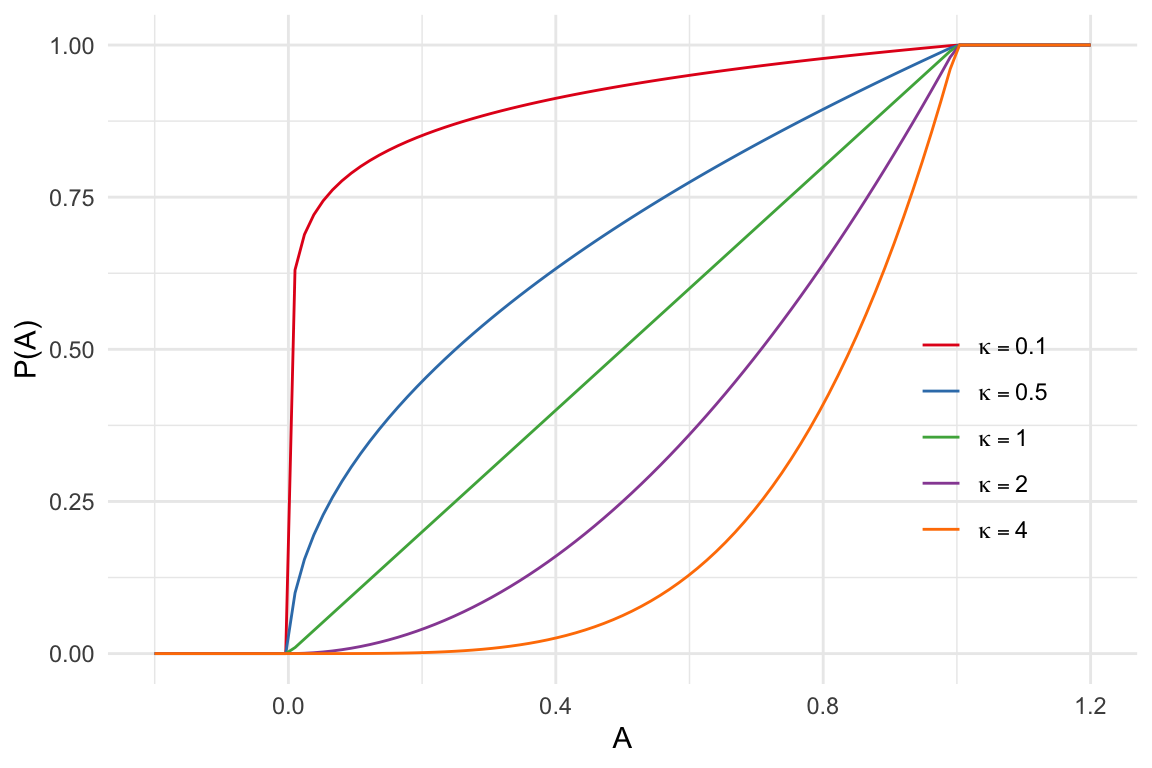
Proposition (continuously differentiable)

Redefine the effort choice problem as $e^{\star }(\alpha ;\pi )\equiv \arg \underset{e}{max}\pi (e)-\alpha e$ where $\alpha =A^{-1}$.

The set of endogenous probabilities is the set $\mathcal{Q}$ of multivalued functions $Q:{\mathbb{R}}_{+}\to [0,1]$ that are decreasing, closed valued, with $\underset{\alpha \to 0}{lim}Q(\alpha )=1$, $Q(\bar{\alpha })=0$ for some $\bar{\alpha }>0$.

For any function $Q\in \mathcal{Q}$ which is continuously differentiable strictly decreasing in the interval $[\underset{―}{\alpha },\bar{\alpha }]$, with $Q(\underset{―}{\alpha })=0$, $Q(\bar{\alpha })=1$, there exists a continuously differentiable function $\pi \in \mathrm{\Pi }$ such that for all $\alpha \in {\mathbb{R}}_{+}$, $Q(\alpha )=\pi (h(\alpha ;\pi ))$.

Proposition proof (continuously differentiable)

Note that $Q(\alpha )=0$ for $\alpha >\bar{\alpha }$, so we may take the boundary condition

$$h(\bar{\alpha })=0$$

Consider the ordinary differential equation

$$\frac{dh}{d\alpha }=\frac{Q^{\prime }}{\alpha },\alpha >0$$

We now define the function $\pi$ as the solution of $\pi (h(\alpha ))=Q(\alpha )$. The function $h$ satisfies the differential equation, which is the first order necessary and sufficient conditions for optimal effort choice problem, namely ${\pi }^{\prime }(h(\alpha ))=\alpha$. Thus, our claim follows.

Logit power

logp_fun <- function(x, kappa) (1 + exp(-x))^(-kappa)
logp_xlim <- c(-5, 5)
ggplot() + 
  geom_function(fun = function(x) logp_fun(x, 0.1), 
                aes(colour = '0.1'), xlim = logp_xlim) + 
  geom_function(fun = function(x) logp_fun(x, 0.5), 
                aes(colour = '0.5'), xlim = logp_xlim) +
  geom_function(fun = function(x) logp_fun(x, 1), 
                aes(colour = '1'), xlim = logp_xlim) +
  geom_function(fun = function(x) logp_fun(x, 2), 
                aes(colour = '2'), xlim = logp_xlim) + 
  geom_function(fun = function(x) logp_fun(x, 4), 
                aes(colour = '4'), xlim = logp_xlim) + 
  labs(x = 'A', y = 'P(A)', colour = '') + 
  scale_colour_brewer(palette = 'Set1', 
                      labels = c(expression(kappa == 0.1), 
                                 expression(kappa == 0.5), 
                                 expression(kappa == 1), 
                                 expression(kappa == 2), 
                                 expression(kappa == 4))) + 
  theme_minimal() + 
  theme(legend.position = c(0.85, 0.4))

Warning: A numeric `legend.position` argument in `theme()` was deprecated in ggplot2
3.5.0.
ℹ Please use the `legend.position.inside` argument of `theme()` instead.

Cutoff power

cutp_fun <- function(x, kappa) pmin(pmax(x, 0)^kappa, 1)
cutp_xlim <- c(-0.2, 1.2)
ggplot() + 
  geom_function(fun = function(x) cutp_fun(x, 0.1), 
                aes(colour = '0.1'), xlim = cutp_xlim) + 
  geom_function(fun = function(x) cutp_fun(x, 0.5), 
                aes(colour = '0.5'), xlim = cutp_xlim) +
  geom_function(fun = function(x) cutp_fun(x, 1), 
                aes(colour = '1'), xlim = cutp_xlim) +
  geom_function(fun = function(x) cutp_fun(x, 2), 
                aes(colour = '2'), xlim = cutp_xlim) + 
  geom_function(fun = function(x) cutp_fun(x, 4), 
                aes(colour = '4'), xlim = cutp_xlim) + 
  labs(x = 'A', y = 'P(A)', colour = '') + 
  scale_colour_brewer(palette = 'Set1', 
                      labels = c(expression(kappa == 0.1), 
                                 expression(kappa == 0.5), 
                                 expression(kappa == 1), 
                                 expression(kappa == 2), 
                                 expression(kappa == 4))) + 
  theme_minimal() + 
  theme(legend.position = c(0.85, 0.4))

Grid search

Logit power

Cutoff power

Figure 1: RMSE heatmap of grid search over $\delta$ and $\kappa$

References

Almlund, Mathilde, Angela Lee Duckworth, James Heckman, and Tim Kautz. 2011. “Personality Psychology and Economics.” In, 4:1–181. Elsevier. https://doi.org/10.1016/B978-0-444-53444-6.00001-8.

Björklund, Anders, and Kjell G. Salvanes. 2011. “Education and Family Background.” In, 201–47. Elsevier. https://doi.org/10.1016/b978-0-444-53429-3.00003-x.

Heckman, James, Jora Stixrud, and Sergio Urzua. 2006. “The Effects of Cognitive and Noncognitive Abilities on Labor Market Outcomes and Social Behavior.” Journal of Labor Economics 24 (3): 411–82.

Ichino, Andrea, Aldo Rustichini, and Giulio Zanella. 2022. “College Education, Intelligence, and Disadvantage: Policy Lessons from the UK in 1960-2004.” http://www.andreaichino.it/wp-content/uploads/IRZ_Sorting.pdf.

Rustichini, Aldo, William G. Iacono, James J. Lee, and Matt McGue. 2023. “Educational Attainment and Intergenerational Mobility: A Polygenic Score Analysis.” Journal of Political Economy 131 (10): 2724–79. https://doi.org/10.1086/724860.

Savage, Jeanne E., Philip R. Jansen, Sven Stringer, Kyoko Watanabe, Julien Bryois, Christiaan A. de Leeuw, Mats Nagel, et al. 2018. “Genome-Wide Association Meta-Analysis in 269,867 Individuals Identifies New Genetic and Functional Links to Intelligence.” Nature Genetics 50 (7): 912–19. https://doi.org/10.1038/s41588-018-0152-6.