| Person-year | Person | |
|---|---|---|
| Panel of genotyped individuals | 5 374 521 | 176 523 |
| Keep graduates only | 3 215 453 | 98 810 |
| Keep graduates with non-missing graduation year | 3 215 453 | 98 810 |
| Graduated between 1970 and 2020 | 3 139 889 | 96 186 |
| Observed between 0 and 25 years since graduation | 1 692 473 | 96 166 |
| Followed from 0 years since graduation | 1 000 872 | 57 956 |
| Followed at least up to age 30 (if secondary) | 963 715 | 51 056 |
Genetic Propensity for Education in Labor Market and Health Trajectories across the Working Life
Origins and persistence of socioeconomic inequality
Choice and luck (“accident of birth”) (Cunha and Heckman 2007)
Genetics and environment interact to shape individual outcomes
Polygenic indices (PGIs) summarise genetic predispositions
Existing evidence on association between PGIs and income remains limited
- static estimates that do not capture income accumulation over the life cycle
- limited evidence on key mediating channels such as employer and occupational sorting
- coarse, self-reported measures of income
This paper
Research questions
- How the genetic endowment influences individual outcomes over the life cycle?
- Role of firms in mediating genetic gradients in income trajectories
What we do
- Link Finnish matched employee-employer registers with genotype data
- Follow graduates annually from graduation up to 25 years later
- Analyse patterns in labour income, firm sorting trajectories by PGI
- analyses the mechanisms underlying differences in SES trajectories
- role of parental PGIs
- contribution of employers and labor market dynamics to the development of inequality
- health functions as an intermediate factor correlated with EA
- DESCRIPTIVE
Contributions
Sociogenomic literature use cross-section with coarse self-reported income: Carvalho (2025), Ghirardi et al. (2024), Rustichini et al. (2023), Barth et al. (2020), Rimfeld et al. (2018)
Distinguish inequality at entry vs divergent career growth
Wage dispersion and worker-firm sorting use estimates of latent worker “skill”: Card et al. (2018), Song et al. (2019), Kline (2024)
Analyse job mobility and firm sorting as mediators of genetic gaps
- Barth et al. (2020): strong correlation between PGI EA and wealth at retirement
- consistent with heterogeneous returns to wealth, \(\uparrow \Pr\) stock investments
- Rustichini et al. (2023): direct genetic and indirect genetic/environment effect on education + assortative mating
- Carvalho (2025): PGI EA strongly correlated with education and occupation choices
- Rimfeld et al. (2018): stronger correlation of education and occupation with PGI EA after Soviet era (\(\Rightarrow\) more meritocratic selection)
- Ghirardi et al. (2024): \(\leq 3875\) NL twins, support compensatory theory (genetics and family wealth as substitutes in education production function)
- continuous administrative measure of income is RARE in sociogenomics
- avoids selective non-response and measurement errors
- large sample
- continuous and long-spanning measure of income
- novel evidence on role of firms and genetics in production of inequality
Preview of results
Favourable genetic endowment (higher PGI for education)
does not explain income level differences at graduation
predicts steeper income trajectory, only among tertiary-educated;
contributes to steeper income path thanks to firm mobility;
acts mostly indirectly through parents (fathers);
is weakly associated with health indices
Data
Genotype data
176 523 genotyped consenting individuals from Finnish biobanks (\(\mathbf{G}_i\))
Polygenic index for years of education (EA-PGI)
weighted sum of genotype vector \(\text{EA-PGI} = \mathbf{G}_i \boldsymbol{\hat{\beta}}\)
measures predisposition to education (including skills and other traits)
\(\boldsymbol{\hat{\beta}}\) (out-of-sample): largest GWAS of educational attainment (Okbay et al. 2022)
Annual registries 1987-2019
Full population coverage
basic records: gender, age, birth year, parents’ ID
education records: highest level, graduation year, field and institution ID
matched employee-employer structure: firm ID, occupation, industry
income records: labour income before tax
healthcare records: we construct Charlson Comorbidity Index
- Many differences can be observed already in-utero,
- STILL graduation has a large impact on life trajectories
- including zero income - NO condition on employment
Analysis sample
Construct sample weights based on full-population data
Empirical approach
Trajectory estimation
\[y_{icmt} = \alpha + \tau_c + \tau_m + \beta_{t} PGI_{i} + \gamma X_{i} + \varepsilon_{icmt}\]
\(y_{icmt}\) outcome of person \(i\) born in year \(c\) observed in year \(m\) at \(t\) years since graduation
\(PGI_i\) standardised EA-PGI
\(X_{i}\) covariates (gender, first ten genetic PCs and biobank indicator)
\(\beta_t\) coefficient of own genetics (+ other environmental factors)
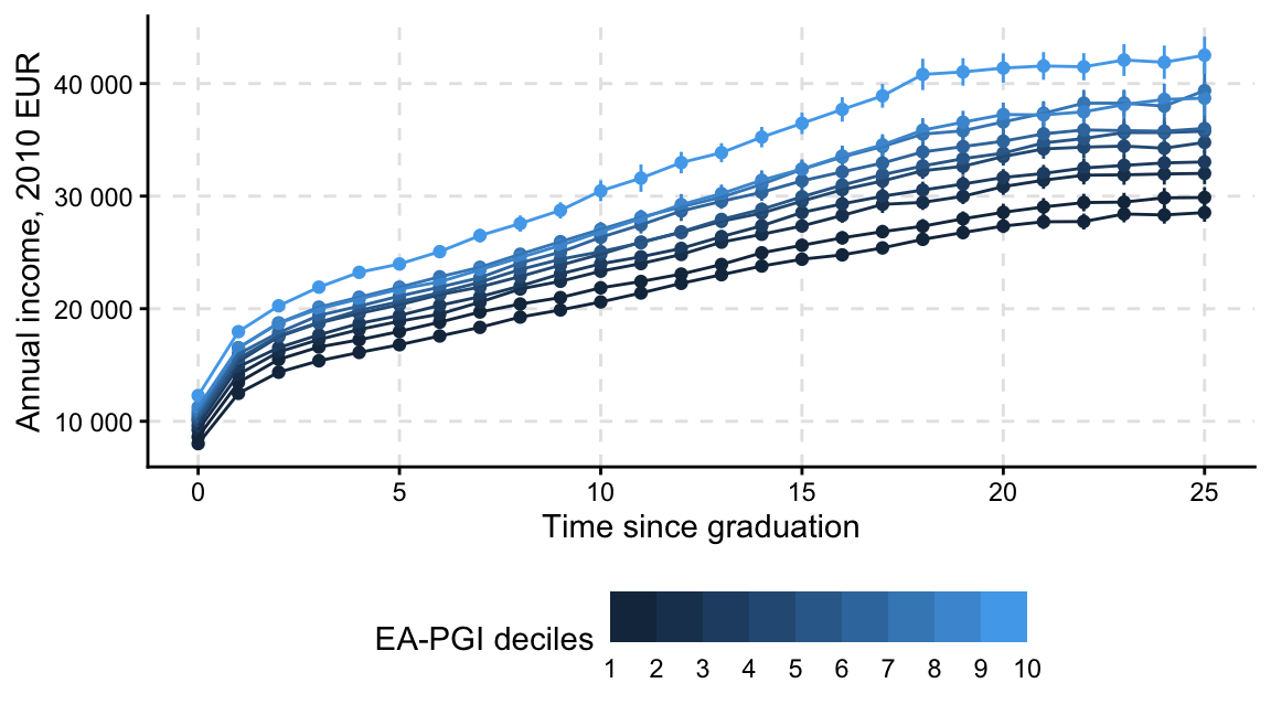
Baseline analysis: average \(\hat{y}_{t}\) at 10th and 90th percentiles of EA-PGI
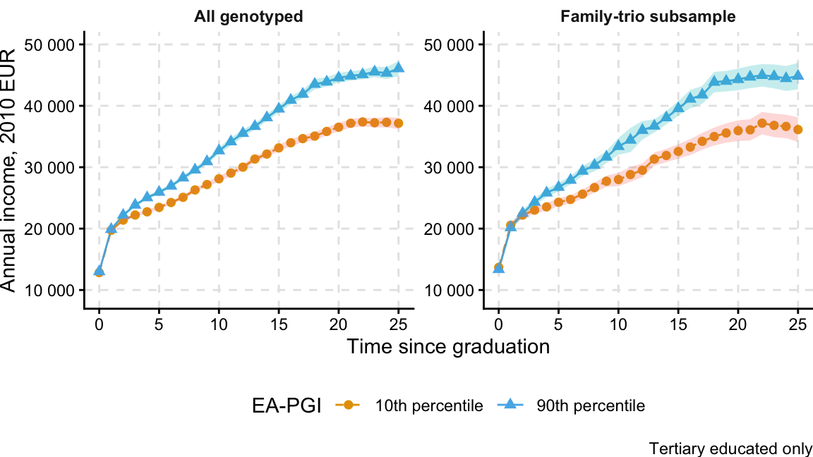
EA-PGI predicts income trajectory, …
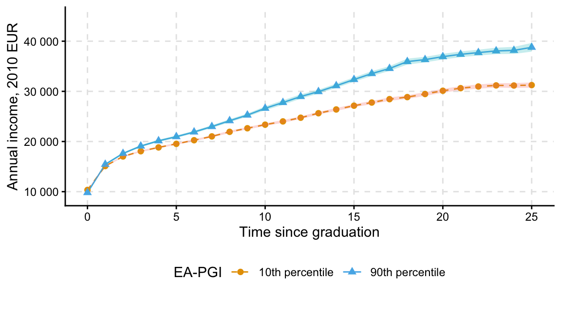
- Initial income levels are nearly identical
- begin to diverge around 3-5 years after graduation
- keep diverging over time (maybe stabilise close to \(t=20\))
EA-PGI predicts income trajectory, …
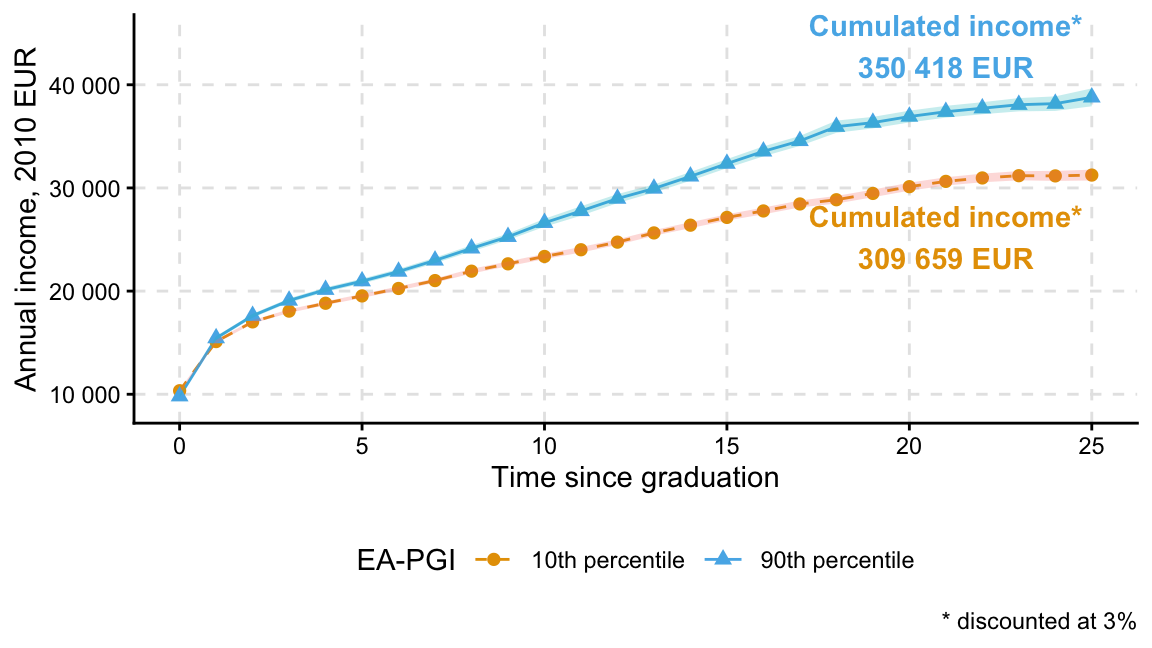
- the gap in discounted lifetime income is about 40,000 EUR
- the gap is 13.2% relative to 10th percentile, or
- about full year of average earnings of top guy at \(t=25\)!
highlight
- initial lack of sorting
- relatively quick employer learning about worker’s productivity
…, but only among tertiary-educated
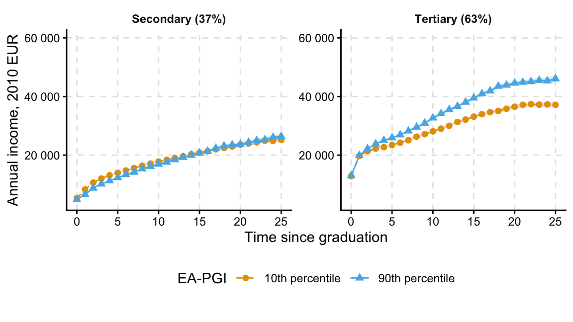
- genetic gradient varies markedly by education
- only present among tertiary-educated (almost 2/3 of sample)
- among-tertiary educated gap stabilises around \(t=15\) (close to peak LM attachment)
- the cumulated income gap is also similar in monetary terms (about €45K)
Firm mobility
High EA-PGI individuals change jobs more rapidly
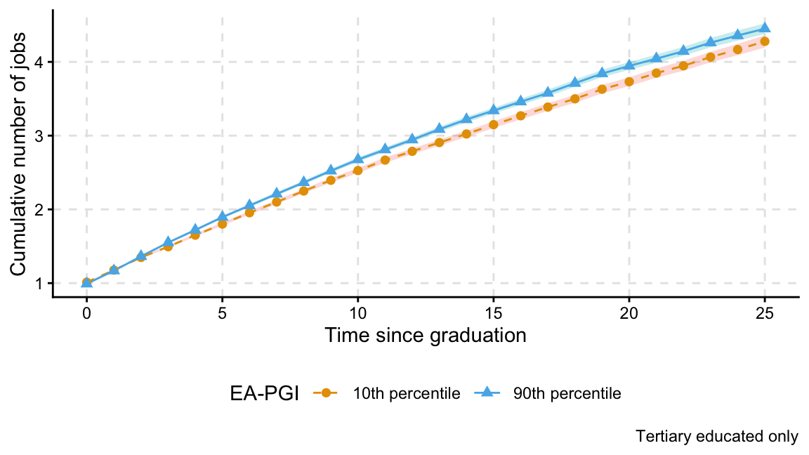
- Individuals at the top of EA-PGI are changing firms slightly more frequently
- Do they switch to better firms when they switch?
AKM decomposition
Using full population registry, estimate
\[y_{it} = \mathbf{X}_{it}\beta + \psi_{J(i, t)} + \theta_i + \varepsilon_{it}\]
\(y_{it}\) monthly labour income of worker \(i\) in year \(t\)
\(\mathbf{X}_{it}\) education fully interacted with calendar year and cubic age polynomial
\(\psi_{J(i, t)}\) firm fixed effect (proxy for firm quality)
\(\theta_i\) worker fixed effect (proxy for worker productivity)
To what extent income gradient is drive by \(\Delta\) productivity?
- higher \(\theta_i\) earn more across all firms relative to some base worker
- higher \(\psi_J\) pay more to all workers relative to some base firm
- holding observables constant (predicted earnings growth due to tenure/age and education)
High EA-PGI individuals transition to higher-quality firms
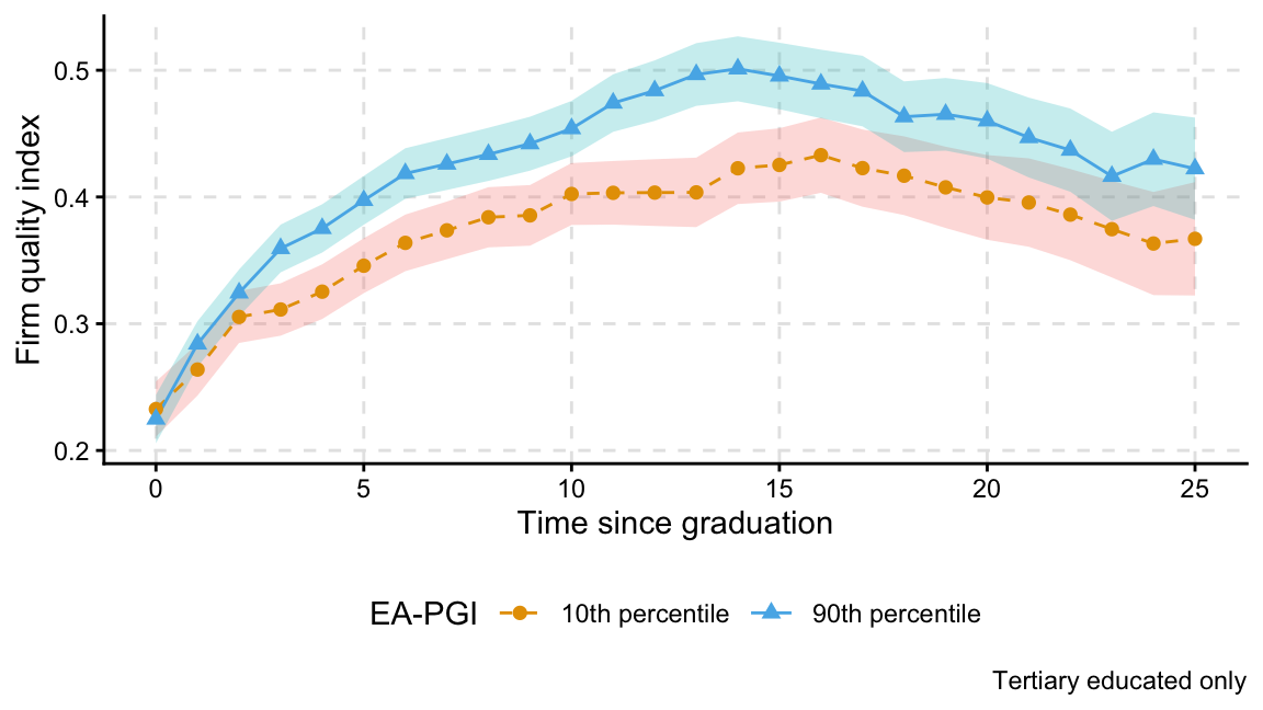
- As soon as there is differential mobility between EA-PGI groups, there is also considerable increase in average firm quality
- Interesting, quality of first employer is same no matter PGI
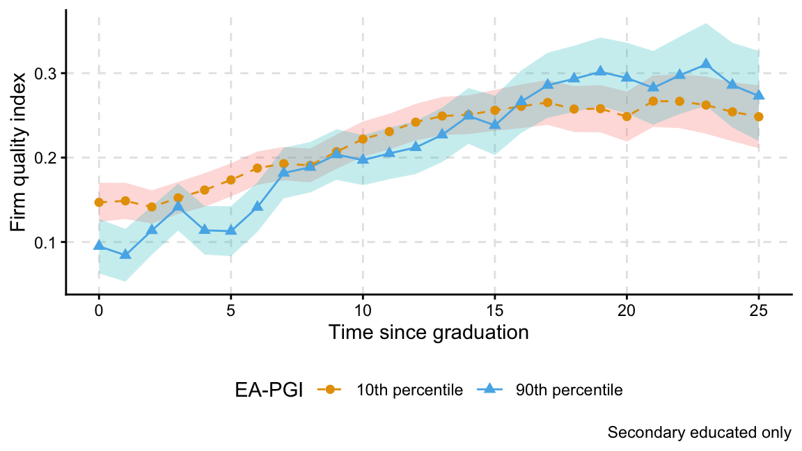
- Firm quality trajectories among secondary-educated are similar across EA-PGI
- Suggest
- greater access to higher-quality higher-paying firms over time
- not so much \(\Delta\) in education, initial LM or frequency of transitions alone
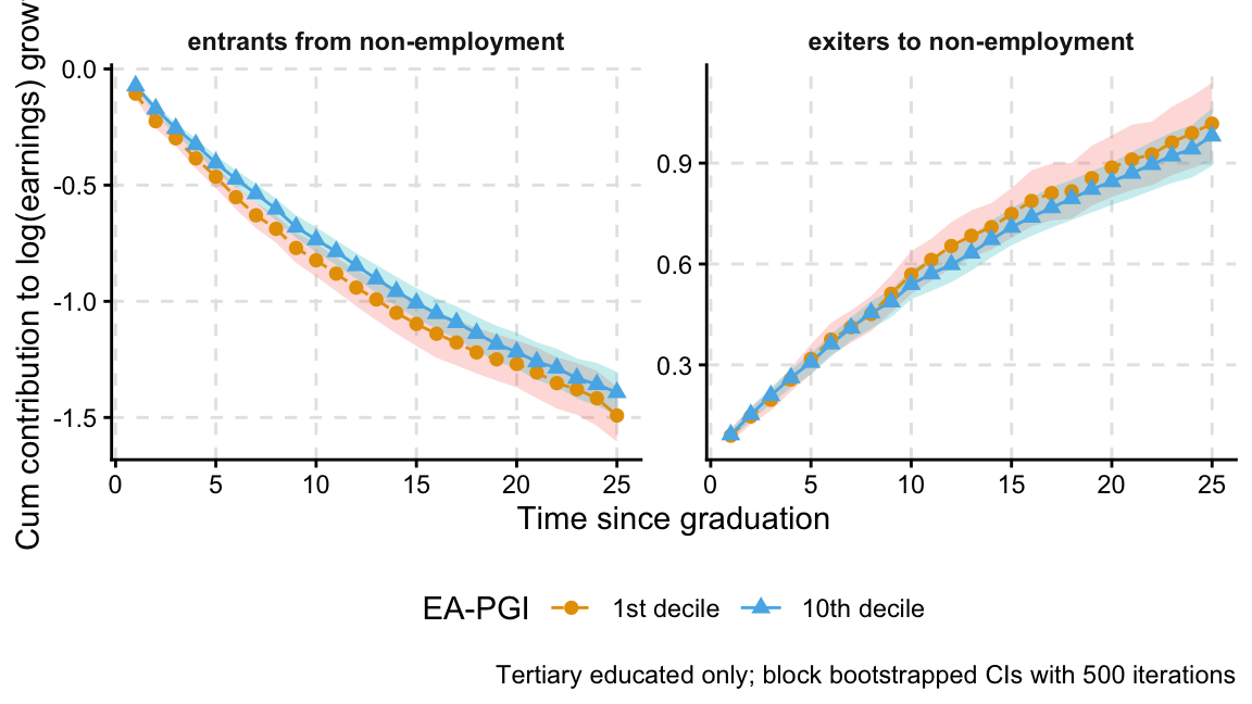
Income disparity by EA-PGI attributable to job changes
Earnings growth decomposition by job mobility (Hahn et al. 2021)
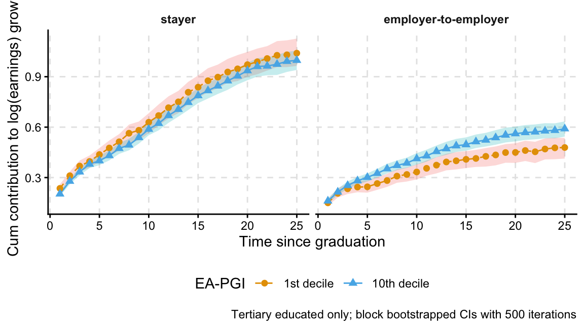
- contribution of between-firm mobility to earnings growth becomes relatively more important over time for top decile EA-PGI
- the gap between top and bottom on the right panel is approximately 10%
- RECALL the gap in DPV income over 25 years is ~13%
- almost no differential contributions among other mobility types
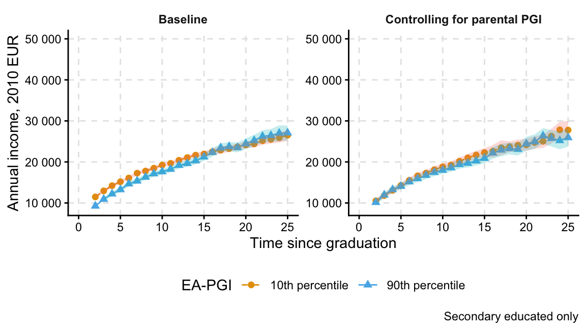
Family trio analysis
Trajectory estimation with parental EA-PGI
Using 12 871 family trios
\[y_{icmt} = \textcolor{gray}{\alpha + \tau_c + \tau_m +} \beta_{t} PGI_{i} + \delta_{t}^m PGI_{i}^m + \delta_t^f PGI_i^f \textcolor{gray}{+ \gamma X_{i} + \varepsilon_{icmt}}\]
\(\beta_t\) captures direct association with genetic endowment
\(\delta_t^m\) and \(\delta_t^f\) reflect both indirect association via parents’ genes and family environment
- Of course, PGI captures not just individual differences in productivity, skills etc
- but also very different environments in early life (more educated parents, higher income families)
- \(\Rightarrow\) to what extent the patterns we’ve seen are really genetically transmitted and have to do something with learning capacity (or some other biological underpinning of skill) versus unequal environment in which skills were being developed?
Income disparity by EA-PGI shrinks by 71% in family analysis
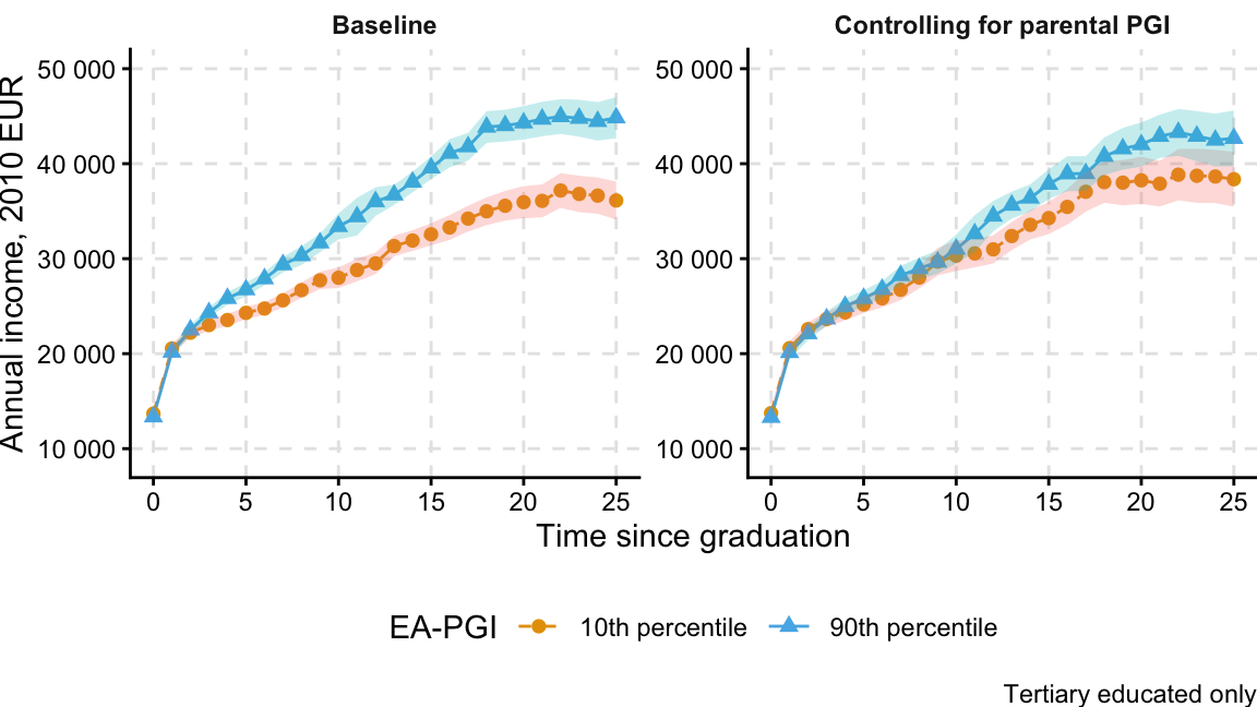
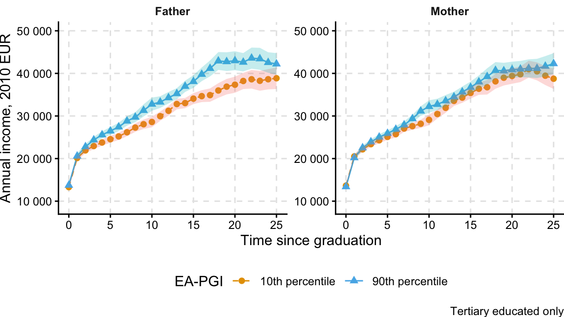
Father EA-PGI predicts children’s income trajectories
Conclusion
Conclusion
Genetic potential most strongly expressed among tertiary-educated people
- Sorting and heterogeneous returns
Large income gap attributed to transitions towards higher-quality employers
- No sorting into first employer: uncertainty about match quality on both sides
- Employer learning and job mobility become more important over time
- Results may partly reflect sorting into better occupations
Indirect genetic associations and parental background highly relevant
- Direct effect of own genes \(\downarrow\) by 71%
- Large part of EA-PGI channel explained by fathers (Del Boca et al. 2013)
Weak association with health indices
Nurfatima Jandarova
Stefano Lombardi
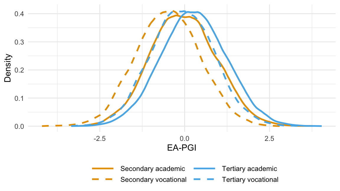
EA-PGI distribution by highest education
Balance table of genotyped graduates
| Population | Genotyped | Reweighted | |||
|---|---|---|---|---|---|
| Mean | Mean | p-val | Mean | p-val | |
| Cohort: 1960-69 | 0.17 | 0.22 | 0.000 | 0.16 | 1.000 |
| Cohort: 1970-79 | 0.34 | 0.36 | 0.000 | 0.34 | 1.000 |
| Cohort: 1980-89 | 0.36 | 0.29 | 0.000 | 0.37 | 1.000 |
| Cohort: 1990-99 | 0.13 | 0.11 | 0.000 | 0.13 | 1.000 |
| Graduation age: 16-20 | 0.36 | 0.31 | 0.000 | 0.36 | 1.000 |
| Graduation age: 21-25 | 0.39 | 0.43 | 0.000 | 0.39 | 1.000 |
| Graduation age: 26-30 | 0.25 | 0.25 | 0.001 | 0.24 | 1.000 |
| Education: secondary | 0.44 | 0.37 | 0.000 | 0.44 | 1.000 |
| Education: tertiary | 0.56 | 0.63 | 0.000 | 0.56 | 1.000 |
| Male | 0.48 | 0.39 | 0.000 | 0.48 | 1.000 |
| Married | 0.10 | 0.13 | 0.000 | 0.11 | 0.000 |
| Rural | 0.24 | 0.25 | 0.712 | 0.25 | 1.000 |
| Income at t=0 | 9 301 | 9 527 | 0.000 | 9 328 | 1.000 |
Average income trajectory by EA-PGI deciles
Weighted income gap
| Pooled | Secondary | Tertiary | ||||
|---|---|---|---|---|---|---|
| Unweighted | Weighted | Unweighted | Weighted | Unweighted | Weighted | |
| 10th percentile | 309 659 | 291 728 | 262 386 | 257 996 | 346 194 | 331 362 |
| (1 306) | (1 286) | (1 429) | (1 501) | (1 944) | (1 920) | |
| 50th percentile | 329 893 | 308 756 | 255 422 | 249 549 | 368 728 | 350 947 |
| ( 857) | ( 832) | (1 116) | (1 157) | (1 137) | (1 105) | |
| 90th percentile | 350 418 | 325 930 | 248 358 | 241 029 | 391 585 | 370 700 |
| (1 591) | (1 525) | (2 120) | (2 185) | (2 006) | (1 938) | |
| Obs. | 51 056 | 51 056 | 18 692 | 18 692 | 32 364 | 32 364 |
AKM summary statistics
| 1987-2003 | 2004-2019 | |
|---|---|---|
| Standard deviation of outcome | 0.5003 | 0.4614 |
| N estimation sample | 16 586 748 | 15 060 995 |
| N worker FE | 1 881 715 | 1 842 564 |
| N firm FE | 126 605 | 50 430 |
| Panel A: Summary of parameter estimates | Panel A: Summary of parameter estimates | Panel A: Summary of parameter estimates |
| RMSE | 0.1693 | 0.1669 |
| Adjusted R2 | 0.8846 | 0.8681 |
| Worker FE | 0.3547 | 0.4868 |
| Firm FE | 0.0458 | 0.0499 |
| Panel B: Share of outcome variance attributed to | Panel B: Share of outcome variance attributed to | Panel B: Share of outcome variance attributed to |
| Cov(worker FE, firm FE) | 0.0269 | 0.0778 |
| Xb and associated covariances | 0.4712 | 0.2703 |
| Residual | 0.1014 | 0.1153 |
- Sample size is huge
- 31.6 mln obs - 3.7 mln workers and 177K firms
- split into two periods: 1987-2003 and 2004-2019
- The indices from two periods are largely consistent with each other (next slide)
AKM fixed effects correlation
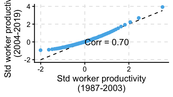
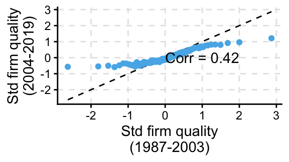
The indices used in main analysis use a combination of the two
- worker observations between 2004-2019 or 1987-2003 will use corresponding \(\hat{\theta}_i\) and \(\hat{\psi}_{J(i, t)}\)
EA-PGI associated with worker productivity
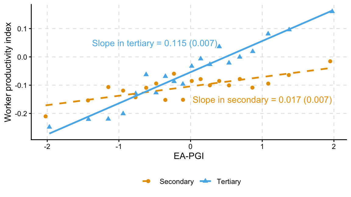
- To what extent income gradient is drive by \(\Delta\) productivity?
- Significant correlation with persistent productivity component
- again only for tertiary
This raises the question whether some high EA-PGI should be encourage to do tertiary edu
Still, this association could be driven by both higher returns and sorting into HE.
EA-PGI association with worker productivity and education
- Large part of the association is driven by education - this suggests large role of sorting into fields/institutions - BUT not all! \(\Rightarrow\) what can the rest relate to? - this could suggest significant role of higher returns to education
of course,
- these are descriptive associations and
- different research strategy is needed to credibly disentangle the two
- this is one of the avenues of follow-up work we are starting with the co-authors
Firm quality trajectory among secondary-educated
Earnings growth decomposition (Hahn et al. 2021)
Accounting framework
\[\Delta \bar{y}_t = \underbrace{E_S ~ \overline{s_t\Delta y_t}}_\text{stayers} + \underbrace{E_Q ~ \overline{q_t \Delta y_t}}_\text{employer-to-employer} + \underbrace{E_N \left(\overline{n_t y_t} - \tilde{y}_t\right)}_\text{entrance from non-empl} - \underbrace{E_R \left(\overline{r_t y_{t - 1}} - \tilde{y}_t\right)}_\text{exit to non-empl}\]
\(y_{it}\) log earnings of worker \(i\) at time \(t\)
\(s_{it} + q_{it} + n_{it} + r_{it} = 1, \forall i, t\)
\(E_k\) employment share of worker type \(k\)
\(\tilde{y}_t\) average income of stayers and employer-to-employer movers
\(s_{it} + q_{it} + n_{it} + r_{it} = 1, \forall i, t\)
\(E_k\) employment share of worker type \(k\)
\(\tilde{y}_t\) average income of stayers and employer-to-employer movers
Contribution of each mobility type to aggregate earnings growth
Contribution of non-employment mobility to earnings growth
Income inequality, firms and occupations
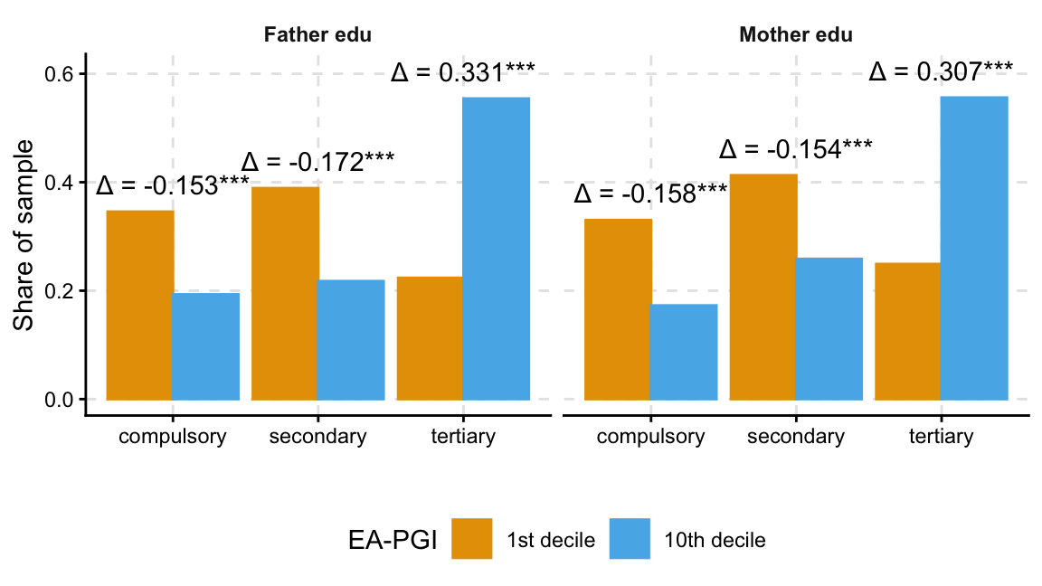
Family background by EA-PGI
Baseline results in family trio subsample
Years of education in family analysis
| Baseline without parental EA-PGI | Controlling for parental EA-PGI | |||
|---|---|---|---|---|
| All family trios | Directly genotyped | All family trios | Directly genotyped | |
| * p < 0.1, ** p < 0.05, *** p < 0.01 | ||||
| Own EA-PGI | 0.553*** | 0.570*** | 0.413*** | 0.441*** |
| (0.016) | (0.027) | (0.026) | (0.040) | |
| Mother EA-PGI | 0.128*** | 0.110*** | ||
| (0.021) | (0.030) | |||
| Father EA-PGI | 0.093*** | 0.095*** | ||
| (0.021) | (0.030) | |||
| Constant | 14.691*** | 13.741*** | 14.641*** | 13.717*** |
| (0.491) | (1.058) | (0.482) | (1.028) | |
| Obs. | 12 871 | 4 586 | 12 871 | 4 586 |
Income gap by EA-PGI of secondary-educated in family analysis
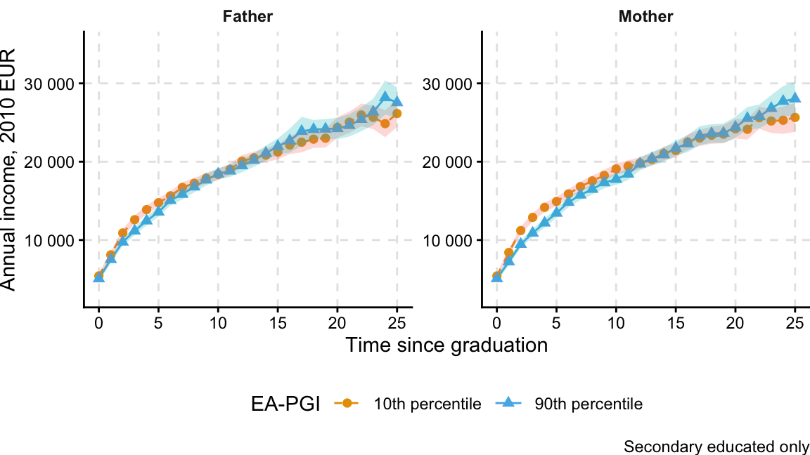
Income gap by parents’ EA-PGI of secondary-educated
Weighted income gap in family analysis
| Pooled | Secondary | Tertiary | ||||
|---|---|---|---|---|---|---|
| Unweighted | Weighted | Unweighted | Weighted | Unweighted | Weighted | |
| 10th percentile | 303 725 | 304 546 | 259 961 | 263 787 | 339 181 | 345 745 |
| (3 906) | (4 417) | (4 621) | (5 261) | (5 690) | (6 559) | |
| 50th percentile | 313 190 | 313 886 | 255 338 | 258 422 | 345 639 | 351 212 |
| (1 697) | (1 981) | (2 154) | (2 388) | (2 320) | (2 755) | |
| 90th percentile | 322 764 | 323 347 | 250 661 | 252 986 | 352 172 | 356 750 |
| (3 934) | (4 502) | (5 294) | (5 717) | (5 198) | (6 114) | |
| Obs. | 12 871 | 12 871 | 5 063 | 5 063 | 7 808 | 7 808 |
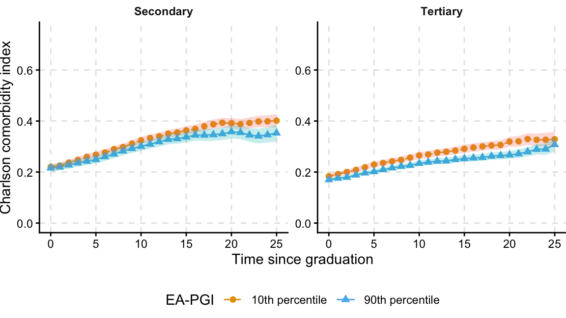
EA-PGI weakly associated with health trajectories
References
Barth, Daniel, Nicholas W. Papageorge, and Kevin Thom. 2020. “Genetic Endowments and Wealth Inequality.” Journal of Political Economy 128 (4): 1474–522. https://doi.org/10.1086/705415.
Card, David, Ana Rute Cardoso, Joerg Heining, and Patrick Kline. 2018. “Firms and Labor Market Inequality: Evidence and Some Theory.” Journal of Labor Economics 36 (S1): S13–70. https://doi.org/10.1086/694153.
Carvalho, Leandro S. 2025. “Genetics and Socioeconomic Status: Some Preliminary Evidence on Mechanisms.” Journal of Political Economy Microeconomics 3 (3): 429–76. https://doi.org/10.1086/732835.
Cunha, Flavio, and James Heckman. 2007. “The Technology of Skill Formation.” American Economic Review 97 (2): 31–47. https://www.aeaweb.org/articles?id=10.1257/aer.97.2.31.
Del Boca, D., C. Flinn, and M. Wiswall. 2013. “Household Choices and Child Development.” The Review of Economic Studies 81 (1): 137–85. https://doi.org/10.1093/restud/rdt026.
Ghirardi, Gaia, Carlos J. Gil-Hernández, Fabrizio Bernardi, Elsje van Bergen, and Perline Demange. 2024. “Interaction of Family SES with Children’s Genetic Propensity for Cognitive and Noncognitive Skills: No Evidence of the Scarr-Rowe Hypothesis for Educational Outcomes.” Research in Social Stratification and Mobility 92 (August): 100960. https://doi.org/10.1016/j.rssm.2024.100960.
Hahn, Joyce K., Henry R. Hyatt, and Hubert P. Janicki. 2021. “Job Ladders and Growth in Earnings, Hours, and Wages.” European Economic Review 133 (April): 103654. https://doi.org/10.1016/j.euroecorev.2021.103654.
Kline, Patrick. 2024. Firm Wage Effects. Vol. 5. Elsevier. https://doi.org/10.1016/bs.heslab.2024.11.005.
Okbay, Aysu, Yeda Wu, Nancy Wang, et al. 2022. “Polygenic Prediction of Educational Attainment Within and Between Families from Genome-Wide Association Analyses in 3 Million Individuals.” Nature Genetics 54 (4): 437–49. https://doi.org/10.1038/s41588-022-01016-z.
Rimfeld, Kaili, Eva Krapohl, Maciej Trzaskowski, et al. 2018. “Genetic Influence on Social Outcomes During and After the Soviet Era in Estonia.” Nature Human Behaviour 2 (4): 269–75. https://doi.org/10.1038/s41562-018-0332-5.
Rustichini, Aldo, William G. Iacono, James J. Lee, and Matt McGue. 2023. “Educational Attainment and Intergenerational Mobility: A Polygenic Score Analysis.” Journal of Political Economy 131 (10): 2724–79. https://doi.org/10.1086/724860.
Song, Jae, David J Price, Fatih Guvenen, Nicholas Bloom, and Till von Wachter. 2019. “Firming up Inequality*.” The Quarterly Journal of Economics 134 (1): 1–50. https://doi.org/10.1093/qje/qjy025.