Canonical model
Overview
Two types of labour: high- and low-skillTypically, high edu and low edu (can be relaxed)
Skill-biased technological change (SBTC)New technology disproportionately \(\uparrow\) high-skill labour productivity
High- and low-skill are imperfectly substitutableTypically, CES production function with elasticity of substitution \(\sigma\)
Competitive labour market
Canonical model
Production function
\[
Y = \left[\left(A_L L\right)^\frac{\sigma - 1}{\sigma} + \left(A_H H\right)^\frac{\sigma - 1}{\sigma}\right]^\frac{\sigma}{\sigma - 1}
\]
\(A_L\) and \(A_H\) are factor-augmenting
\(\sigma \in [0, \infty)\) is the elasticity of substitution
\(\sigma > 1\) gross substitutes\(\sigma < 1\) gross complements\(\sigma = 0\) perfect complements (Leontieff production)\(\sigma \rightarrow \infty\) perfect substitutes\(\sigma = 1\) Cobb-Douglas production
Canonical model
Interpretations
There is only one good and \(H\) and \(L\) are imperfect substitutes in production
There are two goods \(Y_H = A_H H\) and \(Y_L = A_L L\) and consumers have CES utility \(\left[Y_L^\frac{\sigma - 1}{\sigma} + Y_H^\frac{\sigma - 1}{\sigma}\right]^\frac{\sigma}{\sigma - 1}\)
Combination of the two: different sectors produce goods that are imperfect substitutes and \(H\) and \(L\) are employed in both sectors.
Supply of \(H\) and \(L\) is assumed inelastic \(\Rightarrow\) firm problem is sufficient.
Canonical model
Equilibrium wages
\[
\begin{align}
w_L &= A_L^\frac{\sigma - 1}{\sigma} \left[A_L^\frac{\sigma - 1}{\sigma} + A_H^\frac{\sigma - 1}{\sigma}\left(\frac{H}{L}\right)^\frac{\sigma - 1}{\sigma}\right]^\frac{1}{\sigma - 1}\\
w_H &= A_H^\frac{\sigma - 1}{\sigma} \left[A_L^\frac{\sigma - 1}{\sigma}\left(\frac{H}{L}\right)^{-\frac{\sigma - 1}{\sigma}} + A_H^\frac{\sigma - 1}{\sigma}\right]^\frac{1}{\sigma - 1}
\end{align}
\]
Comparative statics:
\(\frac{\partial w_L}{\partial H/L} > 0\) low-skill wage rises with \(\frac{H}{L}\)
\(\frac{\partial w_H}{\partial H/L} < 0\) high-skill wage falls with \(\frac{H}{L}\)
\(\frac{\partial w_i}{\partial A_L} > 0\) and \(\frac{\partial w_i}{\partial A_H} > 0, ~\forall i \in \{L, H\}\) both wages rise with \(A_L\) and \(A_H\)
Canonical model
Skill premium
\[
\frac{w_H}{w_L} = \left(\frac{A_H}{A_L}\right)^\frac{\sigma - 1}{\sigma} \left(\frac{H}{L}\right)^{-\frac{1}{\sigma}}
\]
\(\Delta\) relative supply
\[
\frac{\partial \ln \frac{w_H}{w_L}}{\partial \ln \frac{H}{L}} = -\frac{1}{\sigma} < 0
\]
Relative demand curve is downward-sloping
\[
\frac{\partial \ln\frac{w_H}{w_L}}{\partial \ln\frac{A_H}{A_L}} = \frac{\sigma - 1}{\sigma} \lessgtr 0
\]
Gross substitutes: \(\sigma > 1 \Rightarrow \frac{\partial \ln w_H/ w_L}{\partial \ln A_H / A_L} > 0\)
Gross complements: \(\sigma < 1 \Rightarrow \frac{\partial \ln w_H/ w_L}{\partial \ln A_H / A_L} < 0\)
Cobb-Douglas: \(\sigma = 1 \Rightarrow \frac{\partial \ln w_H/ w_L}{\partial \ln A_H / A_L} = 0\)
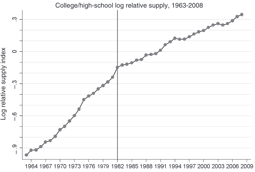
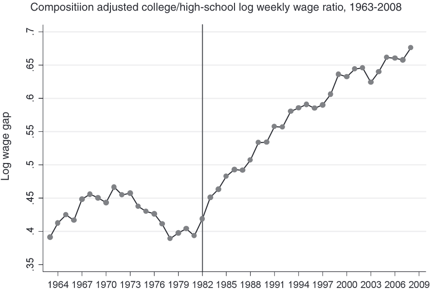
Skill premium and relative supply for a given \(\mathbf{\frac{A_H}{A_L}}\) ! is not surprising:
when supply of high-skilled workers \(\uparrow\) they start performing some of the low-skilled functions
also production of high–skilled goods \(\uparrow\) , now sold at lower price, so also wages of high-skilled workers fall
Also, clear that something must have counteracted this effect given figures at the beginning!
Skill premium and tech shift:
consider Leontieff: tech shift creates excess supply of high-skilled workers \(\Rightarrow w_H \downarrow\)
In general when \(\sigma < 1\) skill premium rises only when \(A_L \uparrow\) (so, tech is skill-replacing )
Tinbergen’s race in the data
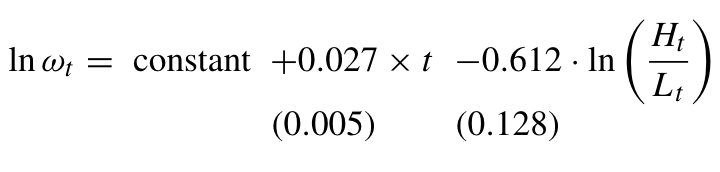
Katz and Murphy (1992 ) The log-equation of skill premium is extremely attractive for empirical analysis
\[
\ln\frac{w_{H, t}}{w_{L, t}} = \frac{\sigma - 1}{\sigma} \ln\left(\frac{A_{H, t}}{A_{L, t}}\right) -\frac{1}{\sigma} \ln \left(\frac{H_t}{L_t}\right)
\]
Assume a log-linear trend in relative productivities
\[
\ln \left(\frac{A_{H, t}}{A_{L, t}}\right) = \alpha_0 + \alpha_1 t
\]
and plug it into the log skill premium equation:
\[
\ln\frac{w_{H, t}}{w_{L, t}} = \frac{\sigma - 1}{\sigma}\alpha_0 + \frac{\sigma - 1}{\sigma} \alpha_1 t -\frac{1}{\sigma} \ln\left(\frac{H_t}{L_t}\right)
\]
Tinbergen’s race in the data
Katz and Murphy (1992 ) Estimated the skill premium equation using the US data in 1963-87
Implies elasticity of substitution \(\sigma \approx \frac{1}{0.612} =\) 1.63
Agrees with other estimates that place \(\sigma\) between 1.4 and 2 (Acemoglu and Autor 2011 )
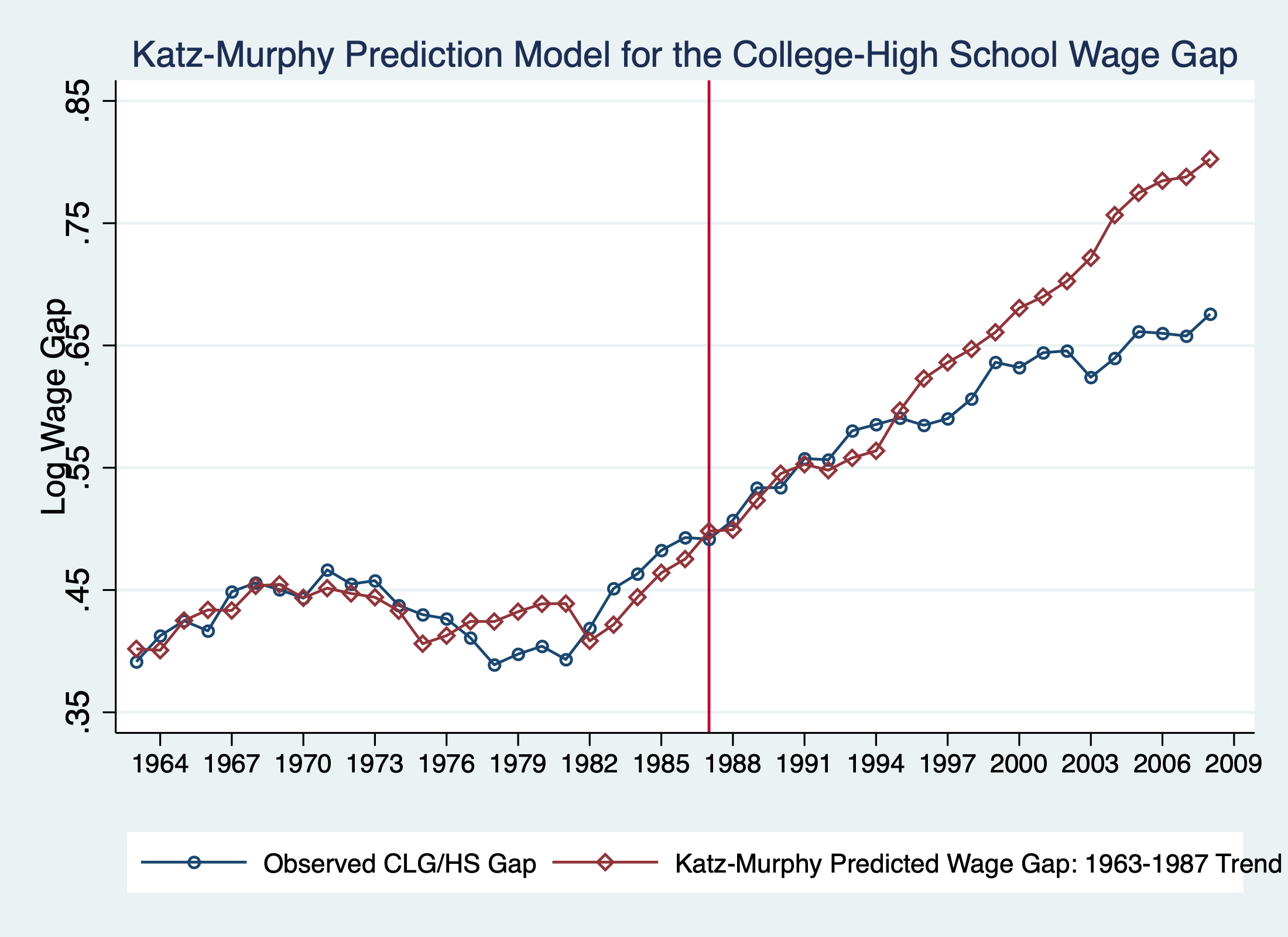
Tinbergen’s race in the data
Very close fit up to mid-1990s, diverge later
Fit up to 2008 implies \(\sigma \approx\) 2.95
Accounting for divergence:
non-linear time trend in \(\ln\frac{A_H}{A_L}\) \(\sigma\) back to 1.8, but implies \(\frac{A_H}{A_L}\) slowed down
differentiate labour by age/experience as well
Canonical model
Summary
Simple link between wage structure and technological change
Attractive explanation for college/no college wage inequality1
Average wages \(\uparrow\) (follows from \(\partial w_i / \partial A_H\) and \(\partial w_i/ \partial A_L\) )
However, the model cannot explain other trends observed in the data:
Falling \(w_L\)
Earnings polarization
Job polarization
Also silent about endogeneous adoption or labour-replacing technology.
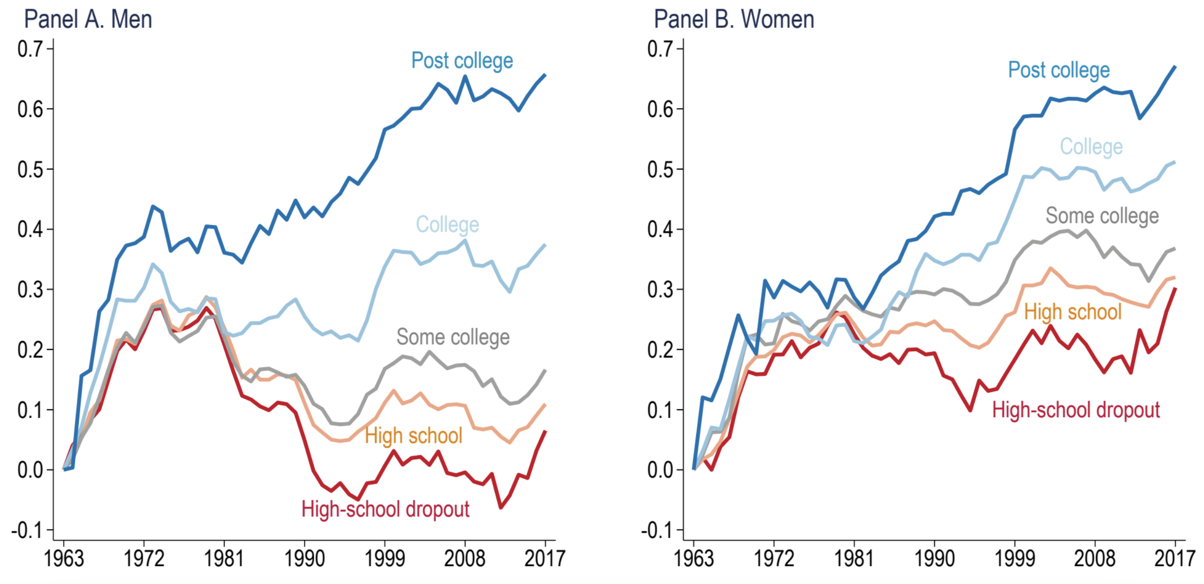
Unexplained trend: falling real wages
Source: Figure 1 in Acemoglu and Restrepo (2022 )
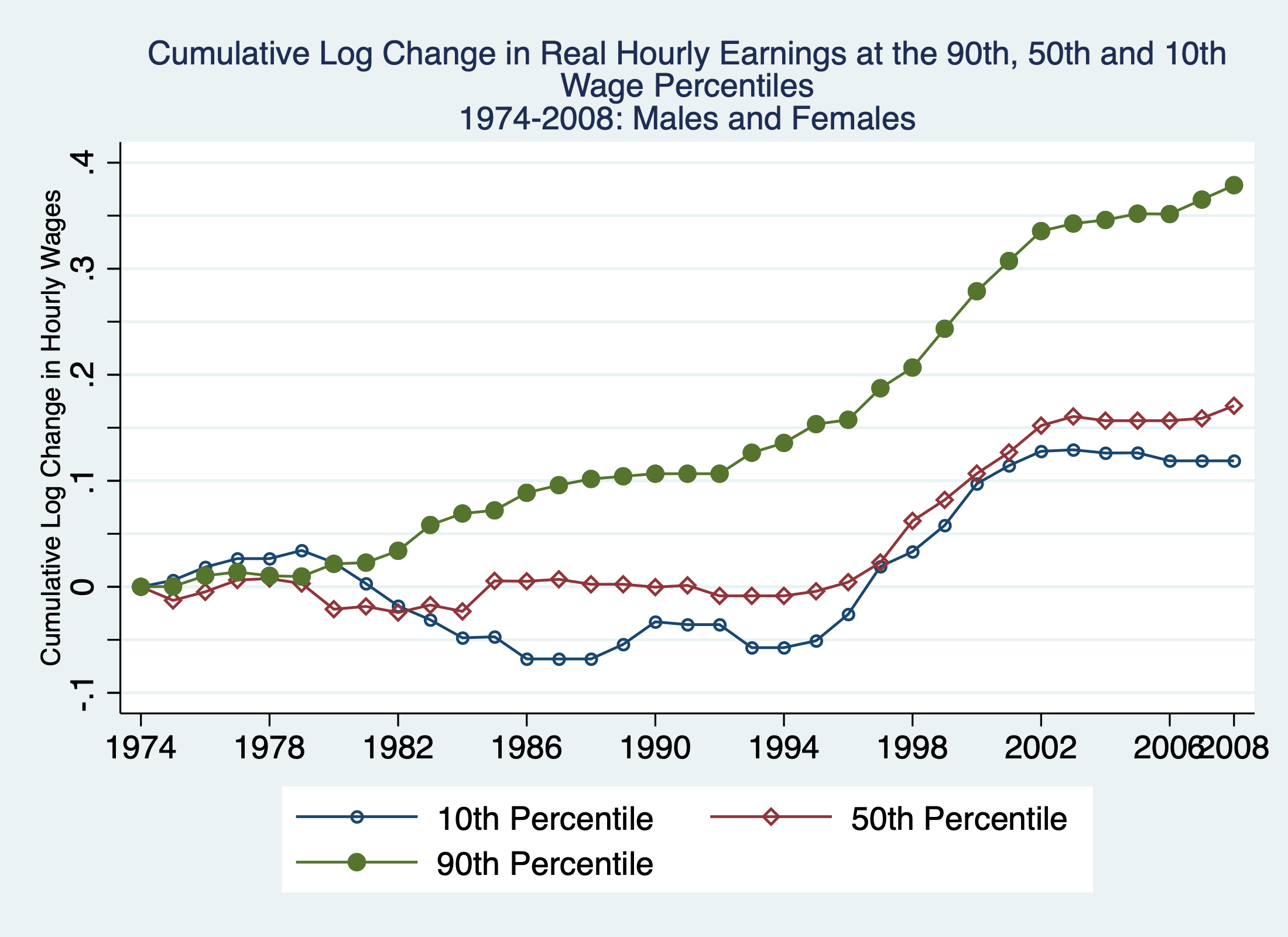
Unexplained trend: earnings polarization
Source: Figure 8 in Acemoglu and Autor (2011 )
The canonical model can explain between group inequality, like college vs non-college workers
But it suggests that within-group inequality in either group moves 1-to-1 with skill premium.
This graph implies that within-group inequalities moved at their own paces.
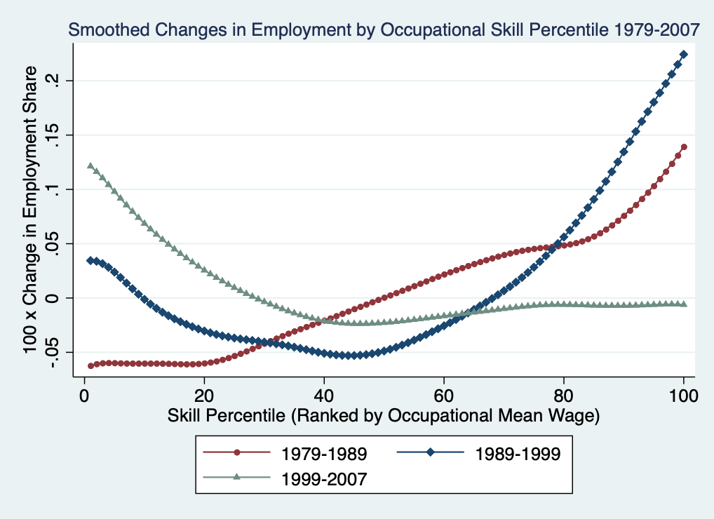
Unexplained trend: job polarization
Source: Figure 10 in Acemoglu and Autor (2011 )
This is just simple, there is absolutely no notion of occupations in the canonical model.
So, no instrument to think about mid-skill mid-job people.
Task-based model
Overview
Task
Skill
Key features:
Tasks can be performed by various inputs (skills, machines)
Comparative advantage over tasks among workers
Multiple skill groups
Consistent with canonical model predictions
Canonical model is a special case: task = skill
Occupations = bundles of tasks
At least 3 skill groups to study earnings polarization
Task-based model
Production function
Unique final good \(Y\) produced by continuum of tasks \(i \in [0, 1]\)
\[
Y = \exp \left[\int_0^1 \ln y(i) \text{d}i\right]
\]
Three types of labour: \(H\) , \(M\) and \(L\) supplied inelastically.
\[
y(i) = A_L \alpha_L(i) l(i) + A_M \alpha_M(i) m(i) + A_H \alpha_H(i) h(i) + A_K \alpha_K(i) k(i)
\]
\(A_L, A_M, A_H\) are factor-augmenting technologies
\(\alpha_L(i), \alpha_M(i), \alpha_H(i)\) are task productivity schedules
\(l(i), m(i), h(i)\) are number of workers by types allocated to task \(i\)
Price of final good is the numeraire \(\Rightarrow \max Y - wL\)
There is now capital in the production function, but no comparative statics about it.
\(\alpha\) terms describe how productive different types are in producing task \(i\)
Hence, each task can be produced by \(L\) , \(M\) and \(H\) , but their comparative advantages are in that task are different!
Task-based model
Comparative advantage assumption
\(\alpha_L(i)/\alpha_M(i)\) and \(\alpha_M(i)/\alpha_H(i)\) are continuously differentiable and strictly decreasing.
Market clearing conditions
\[
\int_0^1 l(i) \text{d}i \leq L \qquad \int_0^1 m(i) \text{d}i \leq M \qquad \int_0^1 h(i) \text{d}i \leq H
\]
Higher task index \(i\) correspond to more complex task in which \(H\) is better than \(M\) is better than \(L\) .
Task-based model
Equilibrium without machines
Given comparative advantage assumption, there exist \(I_L\) and \(I_H\) such that
Note that boundaries \(I_L\) and \(I_H\) are endogenous
This gives rise to the substitution of skills across tasks
Task-based model
Law of one wage
Output price is normalised to 1 \(\Rightarrow \exp\left[\int_0^1 \ln p(i) \text{d}i\right] = 1\)
All tasks employing a given skill pay corresponding wage
\[
\begin{align}
w_L &= \frac{A_L \alpha_L(i)}{p(i)} &\Rightarrow& \qquad l(i) &=& \frac{L}{I_L} &\forall& i < I_L \\
w_M &= \frac{A_M \alpha_M(i)}{p(i)} &\Rightarrow& \qquad m(i) &=& \frac{M}{I_H - I_L} &\forall& I_L < i < I_H \\
w_H &= \frac{A_H \alpha_H(i)}{p(i)} &\Rightarrow& \qquad h(i) &=& \frac{H}{1 - I_H} &\forall& i > I_H
\end{align}
\]
Task-based model
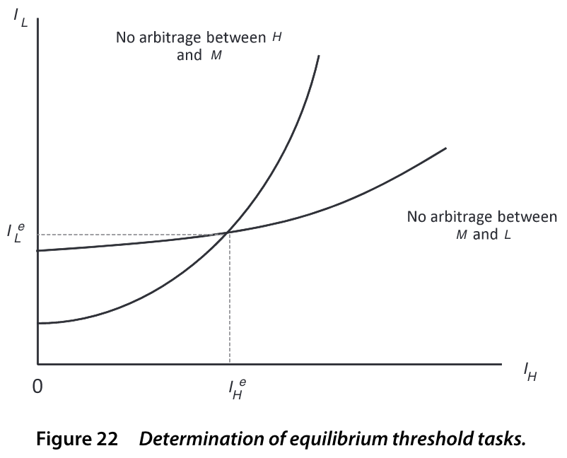
Endogenous thresholds: no arbitrage
Threshold task \(I_H\) : equally profitable to produce with either \(H\) or \(M\) skills
\[
\frac{A_M \alpha_M(I_H) M}{I_H - I_L} = \frac{A_H \alpha_H(I_H) H}{1 - I_H}
\]
Similarly, for \(I_L\) :
\[
\frac{A_L \alpha_L(I_L) L}{I_L} = \frac{A_M \alpha_M(I_L) M}{I_H - I_L}
\]
Task-based model
Endogenous thresholds: no arbitrage
The equilibrium at the intersection because that’s when firm has no incentive to use \(M\) for either of \(L\) or \(H\) tasks. Consider another point along H-M curve: firm is still indifferent between \(H\) and \(M\) for \(I_H\) task. But there will be arbitrage where \(M\) could be more profitable for \(I_L\) task (or \(L\) ).
Task-based model
Comparative statics: wage elasticities
\[
\begin{matrix}
\frac{\text{d} \ln w_H / w_L}{\text{d}\ln A_H} > 0 & \frac{\text{d} \ln w_M / w_L}{\text{d}\ln A_H} < 0 & \frac{\text{d} \ln w_H / w_M}{\text{d}\ln A_H} > 0 \\
\frac{\text{d} \ln w_H / w_L}{\text{d}\ln A_M} \lesseqqgtr 0 & \frac{\text{d} \ln w_M / w_L}{\text{d}\ln A_M} > 0 & \frac{\text{d} \ln w_H / w_M}{\text{d}\ln A_M} < 0 \\
\frac{\text{d} \ln w_H / w_L}{\text{d}\ln A_L} < 0 & \frac{\text{d} \ln w_M / w_L}{\text{d}\ln A_L} < 0 & \frac{\text{d} \ln w_H / w_M}{\text{d}\ln A_L} > 0
\end{matrix}
\]
Consider \(\uparrow A_M\) :
\(M\) more productive \(\Rightarrow ~ \uparrow\) set of medium-skill tasks \(\uparrow I_H\) and/or \(\downarrow I_L\) Since supply is constant, \(\uparrow w_M\) and \(\downarrow w_H, w_L\)
Depending on comparative advantages:
\(\left|\beta^\prime_L(I_L) I_L\right| > \left|\beta^\prime_H(I_H)(1 - I_H)\right| \Rightarrow \frac{w_H}{w_L} \downarrow\) \(\left|\beta^\prime_L(I_L) I_L\right| < \left|\beta^\prime_H(I_H)(1 - I_H)\right| \Rightarrow \frac{w_H}{w_L} \uparrow\)
3a corresponds to when \(L\) have much stronger comparative advantage relative to \(M\) below \(I_L\)
3b on the contrary is when \(H\) have much stronger advantage above \(I_H\) than do \(L\) below \(I_L\) .
When \(A_H \uparrow\) , \(H\) displaces \(M\) directly. There is indirect effect that \(M\) displaces \(L\) , but the indirect effect is small!
Unlike canonical model, changes in \(A\) terms can reduce relative wages! More than that, it is also possible to show they reduce absolute levels of wages too (Wage effects in subsection 4.4)
Task-based model
Task replacing technologies
Assume in \([\underline{I}, \bar{I}] \subset [I_L, I_H]\) machines outperform \(M\) 1 . Otherwise, \(\alpha_K(i) = 0\) .
In this case,
\(w_H / w_M\) increases\(w_M / w_L\) decreases\(w_H / w_L \uparrow \color{#9a2515}{\left(\downarrow\right)}\) if \(\left|\beta^\prime_L(I_L) I_L\right| \stackrel{<}{\color{#9a2515}{>}} \left|\beta^\prime_H(I_H)(1 - I_H)\right|\)
Machines replace \(M \Rightarrow\) demand for \(M \downarrow \Rightarrow w_M \downarrow\)
Even though thresholds move such that \(I_\hat{H} - I_\hat{L} > I_H - I_L\) , the expansion is not large enough to compensate for \(K\) region (I think)
Then, displaced \(M\) can either take up some more tasks that were previously done by \(L\) or \(H\) , but overall demand for \(M\) is down.
Whether or not the displacement is heavier on \(L\) boundary or \(H\) boundary depends on comparative advantages.
Assuming that displacement is larger \(L\) boundary, also demand for \(L\) falls, hence \(w_H/w_L\) rises!
Task-based model
Endogenous supply of skills
Each worker \(j\) is endowed with some amount of each skill \(l^j, m^j, h^j\)
Workers allocate time to each skill given
\[
\begin{align}
&t_l^j + t_m^j + t_h^j \leq 1 \\
&w_L t_l^j l^j + w_M t_m^j m^j + w_H t_h^j h^j
\end{align}
\]
Assuming that \(\frac{h^j}{m^j}\) and \(\frac{m^j}{l^j}\) are decreasing in \(j\) , there exist \(J^\star\left(\frac{w_H}{w_M}\right)\) and \(J^{\star\star}\left(\frac{w_M}{w_L}\right)\)
Comparative statics are more complicated!
But assume that similar to firms pushing \(M\) workers to old \(L\) tasks on the margin, workers too are more elastic at \(J^\star\) than \(J^{\star\star}\) .
Then, the total effect is even stronger for \(\downarrow M\) because less demand from firms and less supply from workers. The effect on \(w_M\) is ambiguous.
However, can’t get nice clean predictions when supply and demand move in different directions.
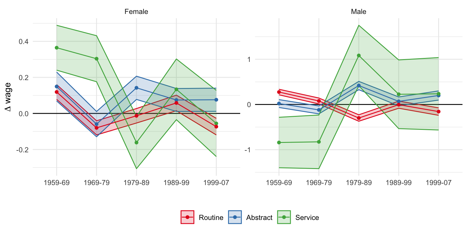
Task-based model
Illustration in the data
Suppose \(A_H \uparrow\) . The model predicts that \(\frac{w_H}{w_M} \uparrow\) and \(\frac{w_M}{w_L} \downarrow\) .
Use occupational specialization at some \(t = 0\) as comparative advantage.
\(\gamma_{sejk}^i\) share of 1959 population employed in \(i\) occupations, \(\forall i \in \{H, M, L\}\)
\[
\Delta w_{sejk\tau} = \sum_t \left[\beta_t^H \gamma_{sejk}^H + \beta_t^L \gamma_{sejk}^L\right] 1\{\tau = t\} + \delta_\tau + \phi_e + \lambda_j + \pi_k + e_{sejk\tau}
\]
Descriptive regression
Stress that since \(H\) is now doing some of what \(M\) used to do, wages per those tasks \(\uparrow\) because \(H\) does it more productively now than \(M\) used to do!
However, \(w_M \downarrow\) because the skill group does less overall.
Wages per task can move in opposite direction than wages per skill!
\(s\) - gender, \(e\) - education, \(j\) - age group, \(k\) - region.
\[
\gamma_{sejk}^H + \gamma_{sejk}^M + \gamma_{sejk}^L = 1
\]
\(\tau\) - decade
Task-based model
Illustration in the data
Source: Table 10 in Acemoglu and Autor (2011 )
Task-based model
Summary
A rich model that can accommodate numerous scenarios
Outsourcing tasks to lower-cost countries
Endogenous technological change
Creation of new tasks
Useful tool to study effect on inequality and job polarization
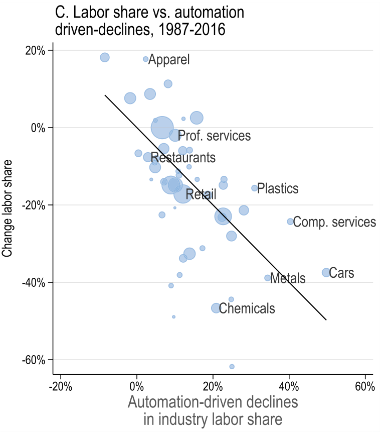
Acemoglu and Restrepo (2022 ) Environment
Multi-sector model with imperfect substitution between production inputs
\[
\text{Task displacement}_g^\text{direct} = \sum_{i \in \mathcal{I}} \omega_g^i \frac{\omega_{gi}^R}{\omega_i^R} \left(-d \ln s_i^{L, \text{auto}}\right)
\]
\(\omega_g^i\) - share of wages earned by worker group \(g\) in industry \(i\) (exposure to industry \(i\) )
\(\frac{\omega_{gi}^R}{\omega_i^R}\) - specialization of group \(g\) in routine tasks \(R\) within industry \(i\)
\(-d \ln s_i^{L, \text{auto}}\) - % decline in industry \(i\) ’s labour share due to automation
attribute 100% of the decline to automation
predict given industry adoption of automation technology
Like in simple exercise, specialization is measured at some \(t_0\) , which here is 1980. So, relative occupation shares in a demographic group “describe” their comparative advantage in that group.
The changes are computed over 1987-2016.
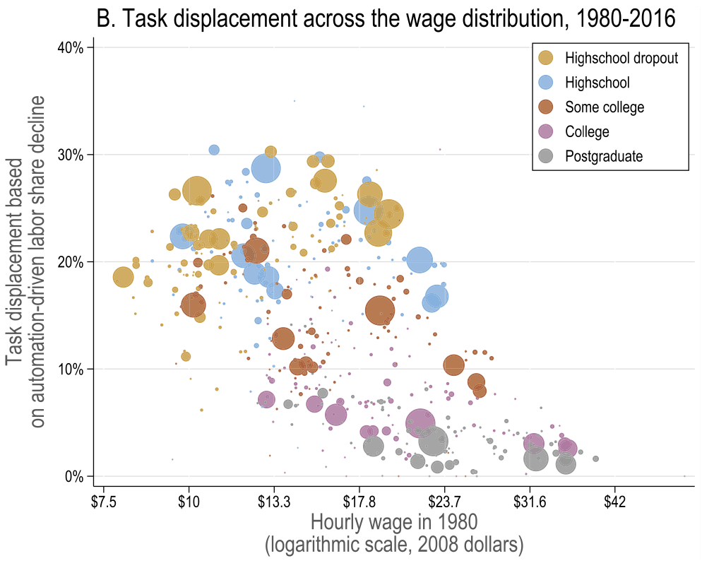
Acemoglu and Restrepo (2022 ) Task displacement
Source: Figure 5
Lower educated groups saw up to 30% decline in their task shares!
The displacement vs initial wage is inverse-U shaped => most of the displacement happened towards the middle
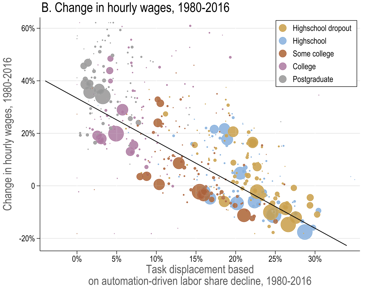
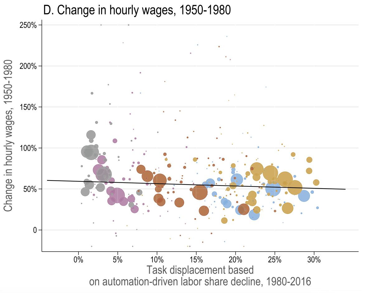
Acemoglu and Restrepo (2022 ) Task displacement and changes in real wages
They verify these observations in a series of reduced form regressions. In particular,
50-70% of changes in wage structure are linked to task displacement and to a much smaller extent to offshoring
they conclude that SBTC without task displacement explains less of variation in the data
they ruled out alternative channels like
However, the reduced form estimates ignore general equilibrium. That is, it assumes
there is no endogenous adjustment of task thresholds at other margins (ripple effects)
no change in industry composition
doesn’t take into account productivity gains
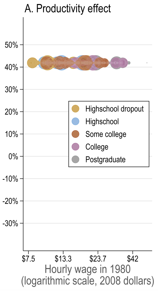
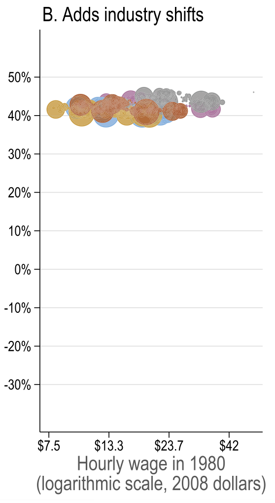
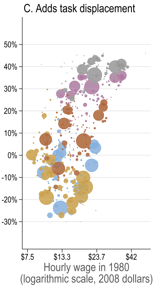
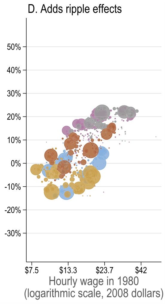
Acemoglu and Restrepo (2022 ) General equilibrium results
Common productivity effect
Changes in industry composition induced by automation\(\Rightarrow\) demand for workers in those sectors goes up
Direct task displacementhigher than reduced form estimates. The direct effect is larger because it does not allow the displaced workers to compete for tasks in other groups. The reduced form estimate did not control for it, hence it picked up some of the ripple effect.
Allowing for ripple effects
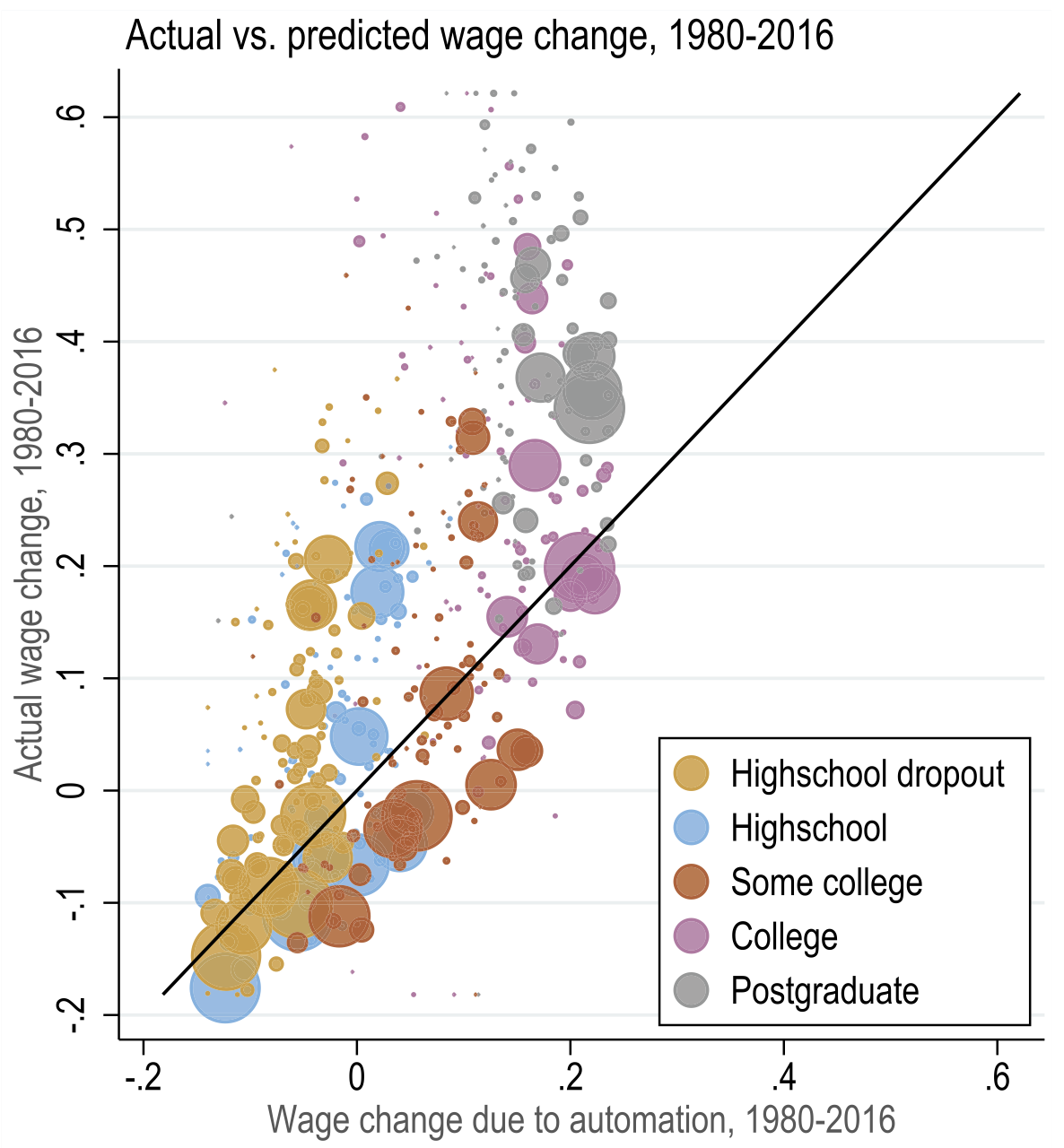
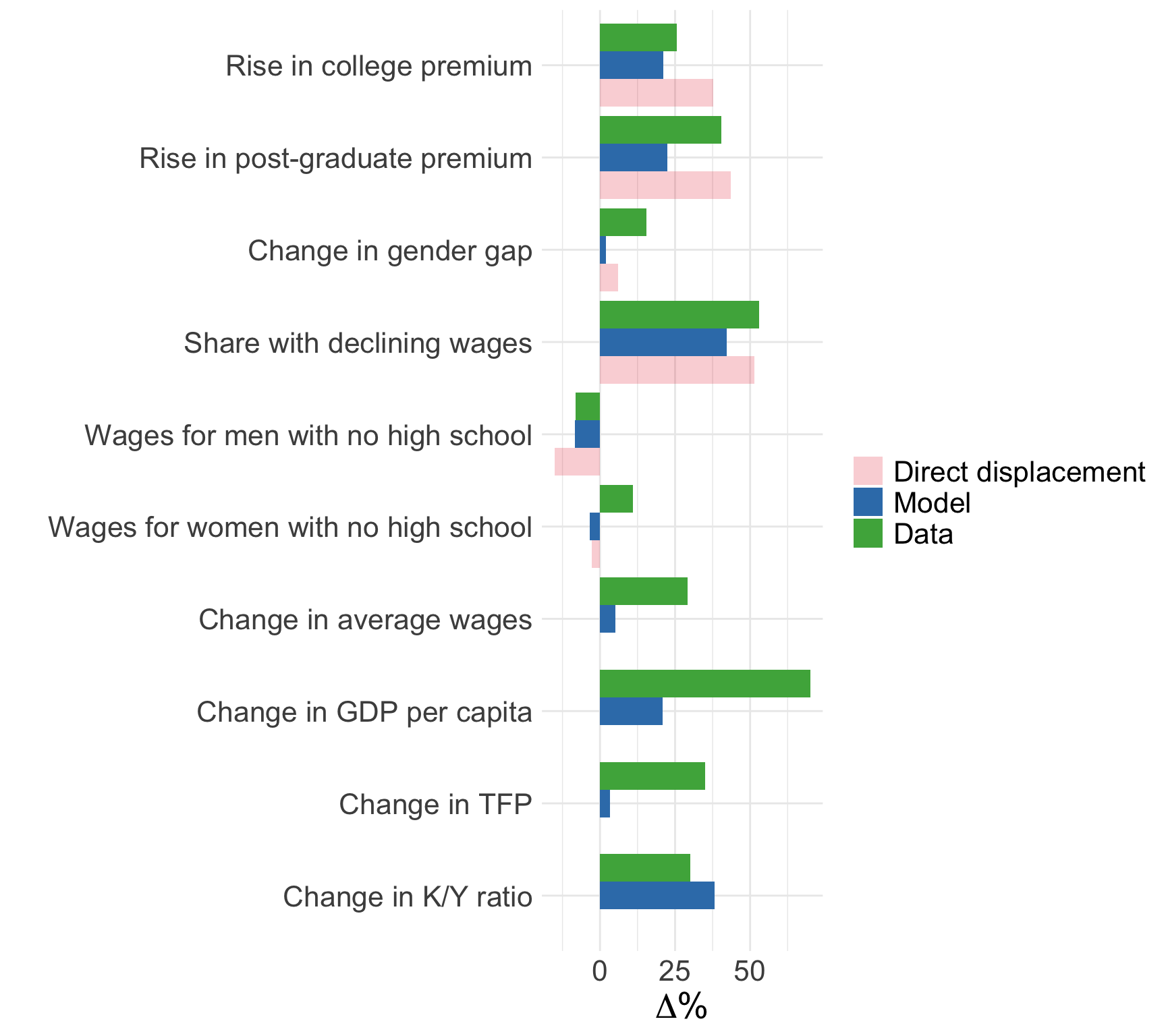
Acemoglu and Restrepo (2022 ) Model fit
The model has close fit to the data everywhere except top of growth distribution
Technology-labour complementarity at the top
Different kinds of jobs (winner-takes-it-all)
Both absent from the model
It also predicts well changes in college premium and wages of men without high school
But it misses big on aggregate things like GDP and TFP
could indicate there were factor-augmenting tech shifts, productivity deepenings, or even new tasks
this wold affect wage levels , but would have little impact on inequality because have shown that inequality is largely attributed to automation
It also suggests that automation-induced investments in the model are in line with data
It also misses on wages of women, which could suggest that supply side ignored so far can also play an important role.
Summary
Two theories linking technological advancements and labour markets
Next: Labour market discrimination
Appendix: derivation of wage equations
The firm problem is to choose entire schedules \(\left(l(i), m(i), h(i)\right)_{i=0}^1\) to
\[
\max PY - w_L L - w_M M - w_H H
\]
Consider FOC wrt \(l(j)\) :
\[
PY \int_0^1 \frac{1}{y(j)} A_L \alpha_L(j) \text{d}i - w_L \int_0^1 \text{d}i = 0
\]
We normalised \(P = 1\) ; therefore, the FOC can be rewritten as
\[
\frac{Y}{y(j)} A_L \alpha_L(j) = w_L
\]
On the next slide, we see that \(\frac{Y}{y(j)} = \frac{1}{p(j)}\) .
Similar argument for \(w_M\) and \(w_H\) .
Appendix: derivation of skill allocations
Numeraire price (\(P=1\) ) is chosen such that \(\frac{y(i)}{Y} = \frac{p(i)}{P} = p(i), \forall i \in [0, 1]\)
Therefore, productivity of \(L\) is \(\frac{Y}{L} = \frac{y(i)}{p(i)L} = \frac{y(j)}{p(j)L}, \forall i \neq j < I_L\)
If we plug in definition of \(y(i)\) and notice that only \(l(i)\) matters when \(i < I_L\) , then
\[
\frac{A_L \alpha_L(i) l(i)}{p(i) L} = \frac{A_L \alpha_L(j)l(j)}{p(j)L}
\]
Given the wage equations in Law of one wage , we know \(\frac{A_L\alpha_L(i)}{p(i)} = \frac{A_L \alpha_L(j)}{p(j)}\) . Therefore, \(l(i) = l(j), \quad \forall i\neq j < I_L\) .
Plug it into the market clearing condition for \(L\)
\[
L = \int_0^{I_L} l(i) \text{d}i = l I_L \quad \Longrightarrow \quad l(i) = l = \frac{L}{I_L}, \forall i < I_L
\]
Similar argument for \(m(i)\) and \(h(i)\) .