5. Education Quality

KAT.TAL.322 Advanced Course in Labour Economics

Nurfatima Jandarova

March 20, 2024

Today

• Education production function
• (Quasi-)Experimental estimations

Education quantity vs quality

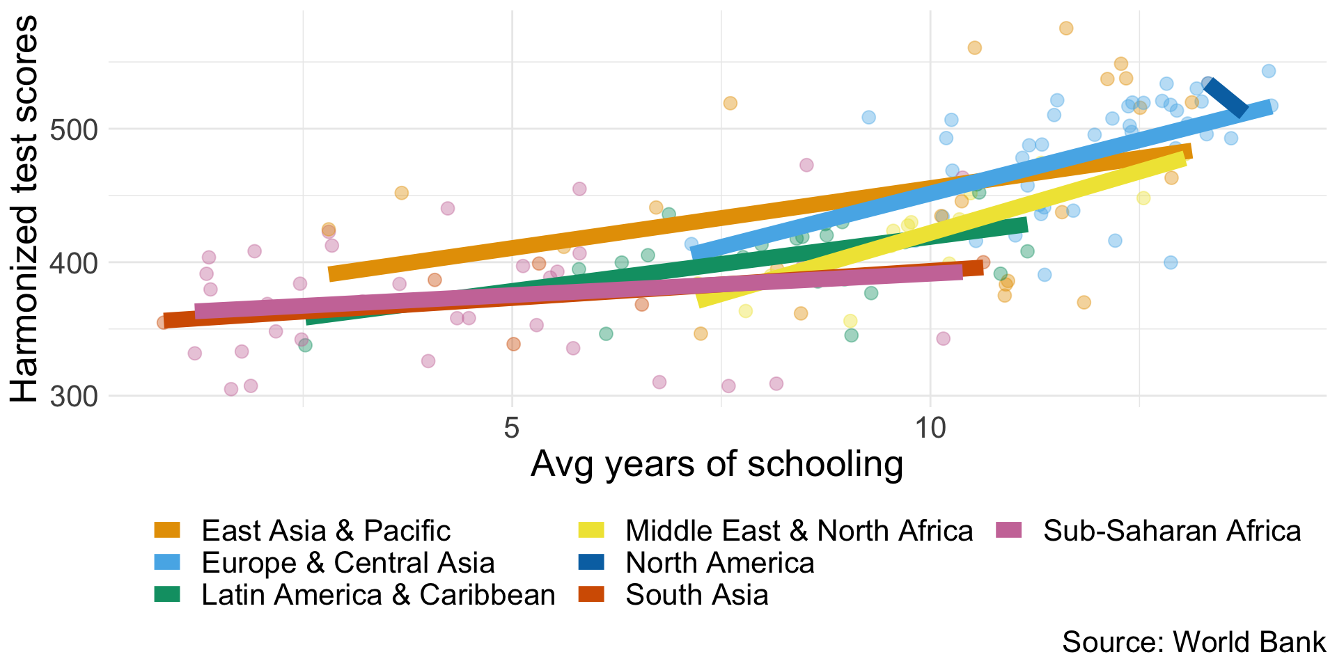
Education quality

Knowledge/productivity doesn’t rise linearly with years of education.

Production process that takes inputs and develops skills.

What are relevant inputs?

What are relevant outputs?

How does production process work?

Education production function

Education production function

Simple framework

Education output of pupil \(i\) in school \(j\) in community \(k\)

\[ q_{ijk} = q(P_i, S_{ij}, C_{ik}) \]

where \(\begin{align}P_i &\quad \text{are pupil characteristics} \\ S_{ij} &\quad \text{are school inputs} \\ C_{ik} &\quad \text{are non-school inputs}\end{align}\)

Education production function

Measures

Output

Years of schooling, standardised test scores, noncognitive skills

Student inputs

Parental characteristics, family income, family size, genetics, patience, effort

School inputs

Teacher characteristics, class sizes, teacher-student ratio, school expenditures, school facilities

Non-school inputs

Peers, local economic conditions, national curricula, regulations, certification rules

Test scores

• Cognitive skill measure

• Skills that are valued in the labour market

• Latent ability vs measured tests

Noncognitive skills

• Itself a multivariate object

• Slowly finding its way to most surveys (Big 5)

• Role of investments in shaping these

Early estimates of school inputs (prior to 1995)

“resources are not closely related to student performance” (Hanushek 2003)

Source: Hanushek (2003), Table 3

Early estimates of school inputs

Methodological concerns

• Static vs cumulative \(\Rightarrow\) levels vs value added

• Endogenous allocation of resources by schools

• Differences in measured output, multiple outputs

• Aggregate policy inputs (curricula, regulation, institutions, etc.)

• Other school inputs (selectivity, teacher biases)

Stronger results in lower quality studies

Outputs: test scores vs continuation, dropout, graduation, earnings

Education production function

Todd and Wolpin (2003)

Achievement of student \(i\) in family \(j\) at age \(a\)

\[ q_{ija} = q_a\left(\mathbf{F}_{ij}(a), \mathbf{S}_{ij}(a), \mu_{ij0}, \varepsilon_{ija}\right) \]

\(\mathbf{F}_{ij}(a)\) history of family inputs up to age \(a\)
\(\mathbf{S}_{ij}(a)\) history of school inputs up to age \(a\)
\(\mu_{ij0}\) initial skill endowment
\(\varepsilon_{ija}\) measurement error in output
\(q_a(\cdot)\) age-dependent production function

Education production function

Todd and Wolpin (2003): Contemporaneous specification

\[ q_{ija} = q_a(F_{ija}, S_{ija}) + \varepsilon_{ija} \]

Strong assumptions:

1. Only current inputs are relevant OR inputs are stable over time
2. Inputs are uncorrelated with \(\mu_{ij0}\) or \(\varepsilon_{ija}\)

Necessary when there (were) severe data limitations

Inputs themselves, as well as their relevance for production function, vary with age of child.

Parental investments depend on (perceptions) of initial endowment.

Education production function

Todd and Wolpin (2003): Value-added specification

\[ q_{ija} = q_a\left(F_{ija}, S_{ija}, \color{#9a2515}{q_{a-1}\left[F_{ij}(a - 1), S_{ij}(a - 1), \mu_{ij0}, \varepsilon_{ij, a - 1}\right]}, \varepsilon_{ija}\right) \]

Typical empirical estimation assumes linear separability and \(q_a(\cdot) = q(\cdot)\):

\[ q_{ija} = F_{ija} \alpha_F + S_{ija} \alpha_S + \gamma q_{ij, a - 1} + \nu_{ija} \]

Additional assumptions implied:

1. Past input effects decay at the same rate \(\gamma\)
2. Shocks \(\varepsilon_{ija}\) are serially correlated with persistence \(\gamma\)

Assume a very simple linear production function with full histories

\[ q_{ija} = X_{ija}\alpha_1 + X_{ij, a - 1}\alpha_2 + \ldots + X_{ij1} \alpha_a + \beta_a \mu_{ij0} + \varepsilon_{ija} \]

Then, same equation at \(a - 1\) is

\[ \gamma q_{ij, a - 1} = \gamma X_{ij, a - 1}\alpha_1 + \ldots + \gamma X_{ij1} \alpha_{a - 1} + \gamma \beta_{a - 1} \mu_{ij0} + \gamma\varepsilon_{ij, a - 1} \]

The difference (or value added) is

\[ q_{ija} - \gamma q_{ij, a - 1} = X_{ija}\alpha_1 + X_{ij, a - 1} \left(\alpha_2 - \gamma \alpha_1\right) + \ldots + X_{ij1}\left(\alpha_a - \gamma \alpha_{a - 1}\right) + \left(\beta_a - \gamma\beta_{a - 1}\right)\mu_{ij0} + \varepsilon_{ija} - \gamma \varepsilon_{ij, a - 1} \]

Therefore, it is clear that for this expression to be equivalent to the above regression equation, the following should hold

\[ \begin{align} \alpha_v &= \gamma \alpha_{v - 1} \\ \beta_v &= \gamma \beta_{v - 1} \end{align}, \qquad \forall v \in 1, \ldots, A \]

In addition, it also highlights that the regression error term \(\nu_{ija} = \varepsilon_{ija} - \gamma\varepsilon_{ij, a - 1}\). So, consistent estimation requires that \(\varepsilon_{ija}\) is serially correlated with persistence exactly equal to \(\gamma\). In that case \(\nu_{ija}\) is white noise and uncorrelated with \(q_{ij, a - 1}\).

If any of these assumptions don’t hold, then estimates will be biased.

Education production function

Todd and Wolpin (2003): Cumulative specification

Still assume linear separability:

\[ q_{ija} = \sum_{t = 1}^a X_{ijt} \alpha_{a - t + 1}^a + \beta_a \mu_{ij0} + \varepsilon_{ij}(a) \]

Estimation strategies:

1. Within-family: \(q_{ija} - q_{i^\prime ja}\) for siblings \(i\) and \(i^\prime\)
2. Within-age: \(q_{ija} - q_{ija^\prime}\) for ages \(a\) and \(a^\prime\)

Each with their own caveats

Within-family

• Siblings observed at different times and/or ages

• Only gets rid of family-specific initial endowments, but not child-specific \(\mu_{ij0} - \mu_{i^\prime j0} \neq 0\)

• So, consistent estimation only possible if input choices are independent of child-specific endowments!

• Furthermore, assumes that there are no spillover effects between siblings. If this assumption is violated then \(\varepsilon_{ij}(a)\) may influence input choices for sibling \(i^\prime\)!

Within-child

• Assumes that \(\beta_a = \beta, \forall a\). Otherwise, differencing across ages does not get rid of initial endowment \(\mu_{ij0}\).

• Assumes that input choices do not depend on past outcomes.

All in all, estimating edu production functions is really really hard!

Education production function

Non-experimental estimations

• Require strong assumptions

  • Some can be relaxed

• Require rich data

(Quasi-)Experimental estimations

• May not recover structural parameters

• Ignore general equilibrium

• Issues with scaling List (2022)

(Quasi-)Experimental estimations

Nature vs nurture

Twin models (ACDE)

Source: Dalliard (2022)

Genetic effects:

• additive \(A\)

• non-additive (dominant) \(D\)

Environment effects:

• common \(C\): by definition correlation = 1

• idiosyncratic \(E\): by definition uncorrelated between twins

Correlation in genetic effects:

• Monozygotic twins

  • these siblings have exactly equal genotypes, both in terms of additive effects and dominant effects (perfect copies)

• Dizygotic twins (as well as normal siblings)

  • in an additive sense, we are interested what is the probability of receiving a given allele from a parent. Answer, 50% (meiosis). At the level of entire genotypes, this means that on average siblings share 50% of their genotypes.

  • For the dominant effect, we want to know what is the chance of receiving dominant allele from both parents. Answer, 50% * 50% = 25% (also meiosis).

Key equations:

\[ \begin{align} VAR &= A^2 + D^2 + C^2 + E^2 \\ COV_{MZ} &= A^2 + D^2 + C^2 \\ COV_{DZ} &= \frac{1}{2} A^2 + \frac{1}{4} D^2 + C^2 \\ h^2 &= \frac{A^2 + D^2}{VAR} \end{align} \]

Identification

The full ACDE model is underidentified: not enough covariances. Thus, have to choose between ACE or DCE models!

Nature vs nurture

Twin models: Polderman et al. (2015)

Meta-analysis of >17,000 twin-analyses (>1,500 cognitive traits)

• 47% of variation due to genetic factors
• 18% of variation due to shared environment

Adoption studies

Fagereng, Mogstad, and Rønning (2021): Korean Norwegian

• Wealth: \(a^2 \approx 58\)% and \(c^2 \approx 37\)%
• Education: \(a^2 \approx 49\)% and \(c^2 \approx 6\)%

Sacerdote (2007): Korean American

• College: \(a^2 \approx 41\)% and \(c^2 \approx 16\)%

• Overall environment factors ~50%

• Most readily amenable to policies \(\Rightarrow\) attractive

• Large policy discussion about school resources

Productivity of school inputs

School spending: review by Handel and Hanushek (2023)

Exogenous variation due to court decisions or legislative action

Quasi-experimental variation in recent studies:

• court-mandated

• legislative action

Besides high variability in estimates, these are not super useful because not clear what exactly money is being spent on

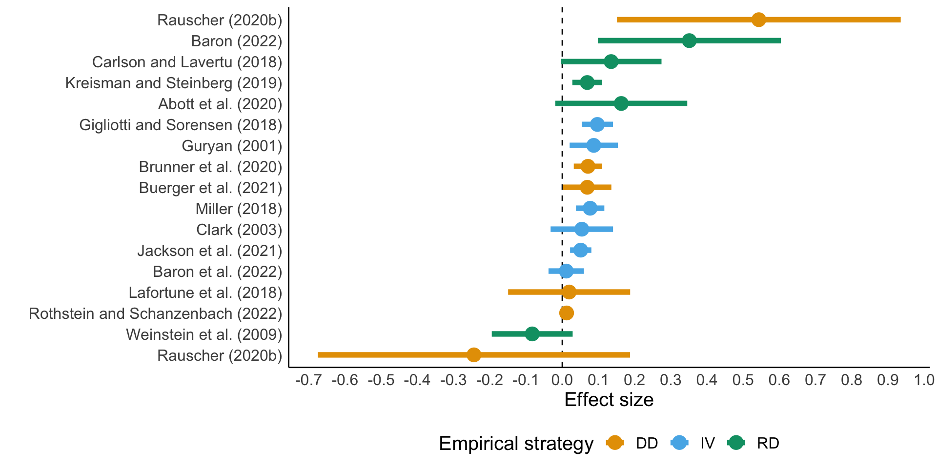
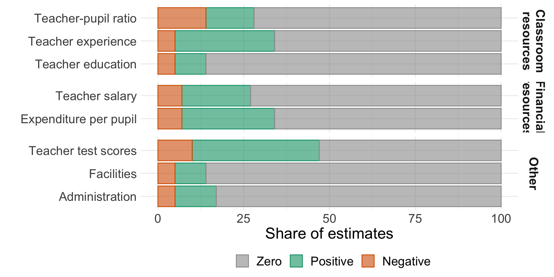
Productivity of school inputs

School spending: review by Handel and Hanushek (2023)

• Large variation of spending effects on test scores

• Not clear how money was used

• Role of differences in regulatory environments

• Similar results for participation rates are all positive (mostly significant)

Bridge the participation results to class sizes on next slide.

Productivity of school inputs

Class size: Angrist and Lavy (1999)

Quasi-experimental variation in Israel: Maimonides rule

Rule from Babylonian Talmud, interpreted by Maimonides in XII century:

If there are more than forty [students], two teachers must be appointed

Sharp drops in class sizes with 41, 81, … cohort sizes in schools

Regression discontinuity design (RDD)

Classical paper!

Productivity of school inputs

Class size: Angrist and Lavy (1999)

Maimonides rule: \(f_{sc} = \frac{E_s}{\text{int}\left(\frac{E_s - 1}{40}\right) + 1}\)

“Fuzzy” RDD

First stage: \(n_{sc} = X_{sc} \pi_0 + f_{sc} \pi_1 + \xi_{sc}\)

Second stage: \(y_{sc} = X_{s}\beta + n_{sc}\alpha + \eta_s + \mu_c + \epsilon_{sc}\)

Productivity of school inputs

Class size: Angrist and Lavy (1999)

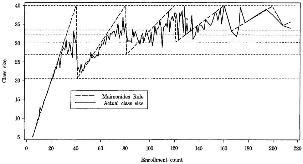
Source: Angrist and Lavy (1999) Figure I

Productivity of school inputs

Class size: Angrist and Lavy (1999)

Source: Angrist and Lavy (1999), Tables IV and V

	Grade 5		Grade 4
	Reading	Math	Reading	Math
Class size	-0.410	-0.185	-0.098	0.095
	(0.113)	(0.151)	(0.090)	(0.114)
Mean score	74.5	67.0	72.5	68.7
SD score	8.2	10.2	7.8	9.1
Obs	471	471	415	415

Productivity of school inputs

Class size: Krueger (1999), Chetty et al. (2011)

Project STAR: 79 schools, 6323 children in 1985-86 cohort in Tennessee

Randomly assigned students into

• small class (13-17 students)

• large class (20-25 students)

\[ Y = \alpha + \beta SMALL + X\delta +\varepsilon \]

Randomization means students between classes are on average similar

\(\boldsymbol{\Rightarrow} \color{#9a2515}{\boldsymbol{\beta}}\) is causal

Krueger (1999) is the classical paper; however, Chetty et al. (2011) provide updated results accounting/fixing several issues with the empirical strategy

• Attrition due to moving away/grade retention

• Some students (not part of initial cohort) joined participating schools in grades 1-3

  • Randomised into small/large classes upon entry

  • Spent < 4 years in the respective classes

• Random assignment into class type (level 1) and classroom (level 2; not documented)

• Some students switched to a different class type

  • assigned to small class: 2.27 years in small class

  • assigned to large class: 0.13 years in small class

Productivity of school inputs

Class size and quality: Chetty et al. (2011)

Source: Chetty et al. (2011) Tables V and VIII

Dependent variable	\(SMALL\)	Class quality1
Test score percentile (at \(t = 0\)), %	4.81 (1.05)	0.662 (0.024)
College by age 27, %	1.91 (1.19)	0.108 (0.053)
College quality, $	119 (96.8)	9.328 (4.573)
Wage earnings, $	4.09 (327)	53.44 (24.84)

Mention fade-out and reemergence

• Almost no effect on test scores beyond the first year in the project (fade-out)

• Significant positive impact on adult earnings (re-emergence)

A potential mechanism of re-emergence: noncognitive skills (next slide)

1. Besides size, experiment generated random variations in class quality (due to teachers, peers, …)

Productivity of school inputs

Class size and quality: Chetty et al. (2011)

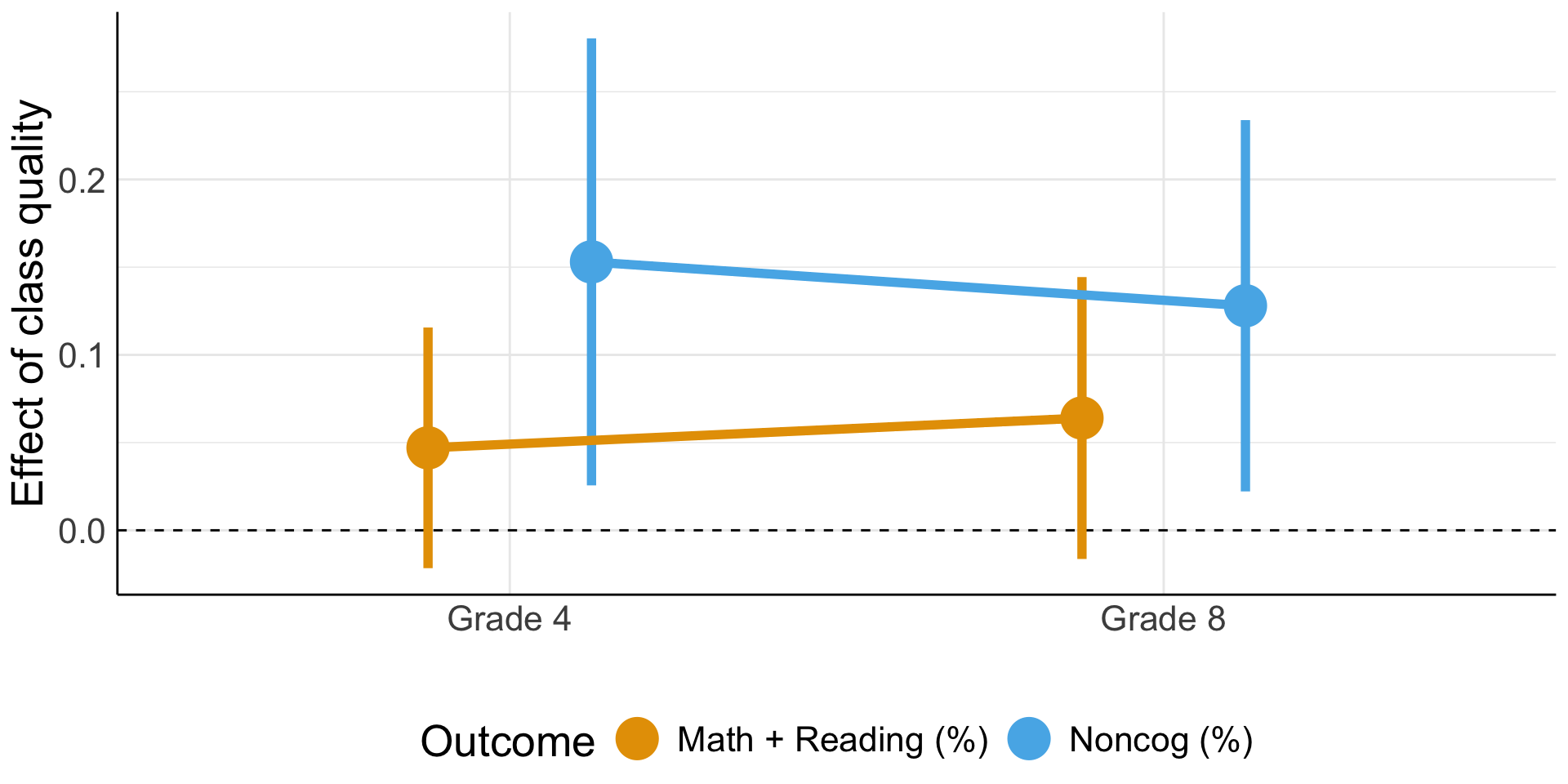
Source: Chetty et al. (2011) Table IX

Productivity of school inputs

Teacher incentives: Fryer (2013)

2-year pilot program in 2007 among lowest-performing schools in NYC

• 438 eligible schools, 233 offered treatment, 198 accepted, 163 control

• Relative rank of schools in each subscore

• Bonus sizes:

  • $3,000/teacher if 100% target
  • $1,500/teacher if 75% target

• Existing studies mostly focus on effort margin, and virtually no paper studies selection margin

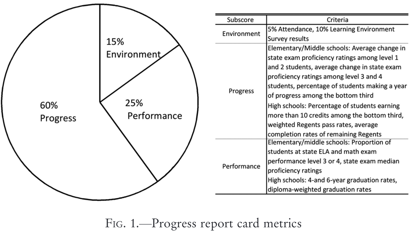
Productivity of school inputs

Teacher incentives: Fryer (2013)

Instrumental variable approach (LATE = ATT):

\[ \begin{align} Y &= \alpha_2 + \beta_2 X + \pi_2 ~ \text{incentive} + \epsilon \\ \text{incentive} &= \alpha_1 + \beta_1 X + \pi_1 ~ \text{treatment} + \xi \end{align} \]

Productivity of school inputs

Teacher incentives: Fryer (2013)

Source: Fryer (2013), Tables 4 and 5

	Elementary	Middle	High
English	-0.010 (0.015)	-0.026 (0.010)	-0.003 (0.043)
Math	-0.014 (0.018)	-0.040 (0.016)	-0.018 (0.029)
Science			-0.018 (0.037)
Graduation			-0.053 (0.026)

Productivity of school inputs

Teacher incentives: Fryer (2013)

• Incentive size was too small (\(\approx 4.1\)% of annual salary)

• Incentive scheme too complex to nudge a certain behaviour

• Bonuses were distributed \(\approx\) equally \(\Rightarrow\) free-riding problem

• Incentivising output vs input

• Effort of existing teachers vs selection into teaching

Productivity of school inputs

Teacher incentives: Biasi (2021)

Change in teacher pay scheme in Wisconsin in 2011:

• seniority pay (SP): collective scheme based on seniority and quals
• flexible pay (FP): bargaining with individual teachers

Main results:

• FP \(\uparrow\) salary of high-quality teachers relative to low-quality

• high-quality teachers moved to FP districts (low-quality to SP)

• teacher effort \(\uparrow\) in FP districts relative to SP

• student test scores \(\uparrow 0.06\sigma\) (1/3 of effect of \(\downarrow\) class size by 5)

• General equilibrium: what happens if all districts switch to FP?

Productivity of non-school inputs

Peer effects: Abdulkadiroğlu, Angrist, and Pathak (2014)

• Prestigious exam schools in Boston and New York

• Students from public schools can transfer at 7th or 9th grades

• Admission based on test scores, GPA and school preference ranking

• Selectivity affects peer composition at either side of the cutoff

Source: Abdulkadiroğlu, Angrist, and Pathak (2014), Figure 1b

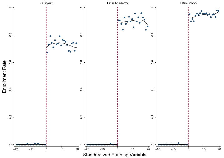
Productivity of non-school inputs

Peer effects: Abdulkadiroğlu, Angrist, and Pathak (2014)

Peer math scores

Proportion Black or Hispanic

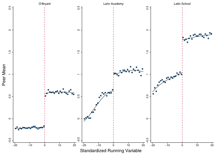
Source: Abdulkadiroğlu, Angrist, and Pathak (2014), Figure 2

Productivity of non-school inputs

Peer effects: Abdulkadiroğlu, Angrist, and Pathak (2014)

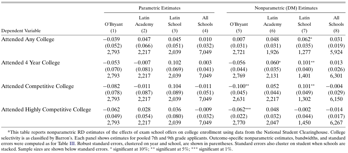
Source: Abdulkadiroğlu, Angrist, and Pathak (2014), Table VI

Productivity of non-school inputs

Peer effects: Abdulkadiroğlu, Angrist, and Pathak (2014)

No effect of peer composition on academic success variables!

Dale and Krueger (2002) study admission into selective colleges in the US

• No effect on average earnings

• Positive effect on earnings of students from low-income families

Kanninen, Kortelainen, and Tervonen (2023): selective schools in Finland

• No effect on high school exit exam score

• Positive effect on university enrollment and graduation rates

• No impact on income

Abdulkadiroğlu, Angrist, and Pathak (2014)

• No visible effect on academic outcomes. Similarly for test scores in later grades.

• External validity: the applicant kids are very different from average kids.

• Preparing for an admission may itself be a productive process/treatment.

• Exposure to clubs and activities may change attitudes, opinions; but these things may not correlate well with outcomes considered in the study.

• The study does not consider labour market outcomes.

  • Maybe networks

Kanninen, Kortelainen, and Tervonen (2023)

Advocate that selective HS changes edu preferences, but not skills!

---

There are other studies that show positive effects of selective schools:

• Pop-Eleches and Urquiola (2013) Romania \(\uparrow\) high-stake test scores

• Jackson (2010) Trinidad and Tobago: large score gains

Overall, there is little consensus on peer effects, selectivity and tracking in education. Some find positive, some find zero effects. Hard to study. A lot of work continues.

Productivity of non-school inputs

Curriculum: Alan, Boneva, and Ertac (2019)

RCT among schools in remote areas of Istanbul

Carefully designed curriculum promoting grit (\(\geq 2\)h/week for 12 weeks)

Treated students are more likely to

• set challenging goals
• exert effort to improve their skills
• accumulate more skills
• have higher standardised test scores

These effects persist 2.5 years after the intervention

• animated videos

• mini case studies

• classroom activities

highlight

• plasticity of brain vs innate ability idea

• role of effort in enhancing skills

• constructive interpretation of setbacks

• importance of goal setting

Productivity of non-school inputs

Curriculum: other evidence

Squicciarini (2020): adoption of technical education in France in 1870-1914

• higher resistance in religious areas, led to lower economic development

Machin and McNally (2008): ‘literacy hour’ introduced in UK in 1998/99

• highly structured framework for teaching

• \(\uparrow\) English and reading skills of primary schoolchildren

• possibility that better curriculum at early stages “frees up” resources at later stages

• not studied the longer-run effects

Summary

• Academic achievement is complex function of student, parent, school and non-school inputs

• Measuring achievement can also be difficult

• Genetic and environmental factors from twin studies almost 50/50

• Large variation in school resource effects (from \(\ll 0\) to \(\gg 0\))

  • How resources are used?
  • Which resources are most effective?

• Studies of class size, teacher incentives, peer effects and curricula

• Another (often overlooked) step is scaling up to the population

Next: Technological shift and labour markets

References

Abdulkadiroğlu, Atila, Joshua Angrist, and Parag Pathak. 2014. “The Elite Illusion: Achievement Effects at Boston and New York Exam Schools.” Econometrica 82 (1): 137–96. https://doi.org/10.3982/ECTA10266.

Alan, Sule, Teodora Boneva, and Seda Ertac. 2019. “Ever Failed, Try Again, Succeed Better: Results from a Randomized Educational Intervention on Grit*.” The Quarterly Journal of Economics 134 (3): 1121–62. https://doi.org/10.1093/qje/qjz006.

Angrist, Joshua D., and Victor Lavy. 1999. “Using Maimonides’ Rule to Estimate the Effect of Class Size on Scholastic Achievement.” The Quarterly Journal of Economics 114 (2): 533–75. https://www.jstor.org/stable/2587016.

Biasi, Barbara. 2021. “The Labor Market for Teachers Under Different Pay Schemes.” American Economic Journal: Economic Policy 13 (3): 63–102. https://doi.org/10.1257/pol.20200295.

Chetty, Raj, John N. Friedman, Nathaniel Hilger, Emmanuel Saez, Diane Whitmore Schanzenbach, and Danny Yagan. 2011. “How Does Your Kindergarten Classroom Affect Your Earnings? Evidence from Project Star *.” The Quarterly Journal of Economics 126 (4): 1593–1660. https://doi.org/10.1093/qje/qjr041.

Dale, Stacy Berg, and Alan B. Krueger. 2002. “Estimating the Payoff to Attending a More Selective College: An Application of Selection on Observables and Unobservables.” The Quarterly Journal of Economics 117 (4): 1491–1527. https://www.jstor.org/stable/4132484.

Dalliard. 2022. “Classical Twin Data and the ACDE Model.” Human Varieties. July 18, 2022. https://humanvarieties.org/2022/07/18/classical-twin-data-and-the-acde-model/.

Fagereng, Andreas, Magne Mogstad, and Marte Rønning. 2021. “Why Do Wealthy Parents Have Wealthy Children?” Journal of Political Economy 129 (3): 703–56. https://doi.org/10.1086/712446.

Fryer, Roland G. 2013. “Teacher Incentives and Student Achievement: Evidence from New York City Public Schools.” Journal of Labor Economics 31 (2): 373–407. https://doi.org/10.1086/667757.

Handel, Danielle Victoria, and Eric A. Hanushek. 2023. “US School Finance: Resources and Outcomes.” In Handbook of the Economics of Education, 7:143–226. Elsevier. https://doi.org/10.1016/bs.hesedu.2023.03.003.

Hanushek, Eric A. 2003. “The Failure of Input‐based Schooling Policies.” The Economic Journal 113 (485): F64–98. https://doi.org/10.1111/1468-0297.00099.

Kanninen, Ohto, Mika Kortelainen, and Lassi Tervonen. 2023. “Long-Run Effects of Selective Schools on Educational and Labor Market Outcomes.” VATT Working Papers. Helsinki. December 2023. https://www.doria.fi/bitstream/handle/10024/188274/vatt-working-papers-161-long-run-effects-of-selective-schools-on-educational-and-labor-market-outcomes.pdf?sequence=1&isAllowed=y.

Krueger, Alan B. 1999. “Experimental Estimates of Education Production Functions.” The Quarterly Journal of Economics 114 (2): 497–532. https://www.jstor.org/stable/2587015.

List, John A. 2022. The Voltage Effect: How to Make Good Ideas Great and Great Ideas Scale. 1st ed. New York: Crown Currency.

Machin, Stephen, and Sandra McNally. 2008. “The Literacy Hour.” Journal of Public Economics 92 (5): 1441–62. https://doi.org/10.1016/j.jpubeco.2007.11.008.

Polderman, Tinca J. C., Beben Benyamin, Christiaan A. de Leeuw, Patrick F. Sullivan, Arjen van Bochoven, Peter M. Visscher, and Danielle Posthuma. 2015. “Meta-Analysis of the Heritability of Human Traits Based on Fifty Years of Twin Studies.” Nature Genetics 47 (7): 702–9. https://doi.org/10.1038/ng.3285.

Sacerdote, Bruce. 2007. “How Large Are the Effects from Changes in Family Environment? A Study of Korean American Adoptees*.” The Quarterly Journal of Economics 122 (1): 119–57. https://doi.org/10.1162/qjec.122.1.119.

Squicciarini, Mara P. 2020. “Devotion and Development: Religiosity, Education, and Economic Progress in Nineteenth-Century France.” American Economic Review 110 (11): 3454–91. https://doi.org/10.1257/aer.20191054.

Todd, Petra E., and Kenneth I. Wolpin. 2003. “On the Specification and Estimation of the Production Function for Cognitive Achievement.” The Economic Journal 113 (485): F3–33. https://www.jstor.org/stable/3590137.