| 1930 cohort | 1940 cohort | |
|---|---|---|
| r | 0.076 | 0.095 |
| (0.029) | (0.022) | |
| Weak IV F-stat | 1.6 | 3.2 |
4. Human Capital
KAT.TAL.322 Advanced Course in Labour Economics
Nurfatima Jandarova
March 14, 2024
Human capital
Labour heterogeneity is important for labour supply and demand.
Human capital includes education, training, health investments.
First references as early as Adam Smith; formalised by Becker in 1960s.
Overview
Overview
Human capital is an investment
- benefit: gain in earnings
- cost: tuition, foregone earnings, psychological costs
Two main camps for source of gain in earnings:
gain in productivity
signalling
Human capital production function
Typically, univariate (years of education), but can be complex function of
Innate skills (e.g., genetics)
Parental investments (e.g., day care, time spent with children, tutors)
Schooling/formal education
- Quantity (e.g., high school vs university)
- School quality (e.g., teacher quality, expenditure per student)
- Differences in curricula/fields (e.g., STEM vs arts)
Peers (e.g., at school, at work)
On-the-job training (e.g., general vs specific skills)
Productive human capital investments
Basic model
Assume education choice \(S \in \{HS, C\}\)
Worker with \(s\) produces \(Y_s\) goods when employed by a firm, \(\forall s \in S\).
Perfect competition ensures that \(W_{HS} = Y_{HS}\) and \(W_C = Y_C\)
Assume cost of education given by function \(\eta(S)\)
Then choose college if marginal benefit outweighs marginal cost
\[ S = C \iff \color{#288393}{W_{C} - W_{HS}} \geq \color{#9a2515}{\eta(C) - \eta(HS)} \]
Lifecycle model: simplified Ben-Porath (1967)
- Divide time between schooling/training \(\sigma(t)\) and working \(1 - \sigma(t)\)
- Law of motion of HC: \(\dot{h}(t) = \theta \sigma(t)h(t)\)
- Production function per worker: \(y(t) = Ah(t)\) = wage
- Assume linear utility and no utility cost of \(\sigma(t)\)
\[ \Omega = \int_0^T \left(1 - \sigma(t)\right) Ah(t)e^{-rt} dt \qquad \text{s.t. HC law of motion} \]
Marginal return to HC effort \(\sigma(t)\) is
\(\frac{\partial \Omega}{\partial \sigma(t)} = -Ah(t)e^{-rt} + \int_0^T \left(1 - \sigma(z)\right) A\frac{\partial h(z)}{\partial \sigma(t)} e^{-rz} dz\)
\(\frac{\partial \Omega}{\partial \sigma(t)} = \color{#8e2f1f}{\underbrace{-Ah(t)e^{-rt}}_\text{foregone earnings}} + \color{#288393}{\underbrace{A\theta\int_t^T \left(1 - \sigma(z)\right) h(z) e^{-rz} dz}_\text{discounted future payoff}}\)
Lifecycle model: simplified Ben-Porath (1967)
Optimal effort is zero at low efficiency \(\theta\) and high discount rate \(r\)
The change in marginal return over time is given by
\[ \frac{d}{dt}\left(\frac{\partial \Omega}{\partial \sigma(t)}\right) = A h(t) e^{-rt}(r - \theta) \]
If \(r > \theta\), then marginal return \(\uparrow\) over time, but is negative at \(T\):
\[ \frac{\partial \Omega}{\partial \sigma(T)} = -Ah(T)e^{-rT} < 0 \]
Hence, marginal return at every period is negative \(\Rightarrow \sigma^*(t) = 0 \quad \forall t\).
Lifecycle model: simplified Ben-Porath (1967)
Optimal effort when efficiency \(\theta\) is high or discount rate \(r\) is low
Marginal return \(\downarrow\) over time \(\Rightarrow\) may exist \(t = s\) such that \(\frac{\partial \Omega}{\sigma(s)} = 0\)
- initial investment into education \(\sigma^*(t) = 1, \quad \forall t \leq s\)
- work rest of the time \(\sigma^*(t) = 0, \quad \forall t > s\)
- study longer if \(\theta\) higher
\[s = \begin{cases}T + \frac{1}{r}\ln\left(\frac{\theta - r}{\theta}\right) & \text{if } \theta \geq \frac{r}{1 - e^{-rT}} \\ 0 & \text{otherwise}\end{cases}\]
Lifecycle model: Ben-Porath (1967)
Allows for human-capital depreciation and on-the-job training
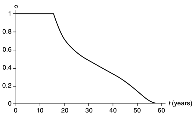
Source: Figure 4.9 from Cahuc (2004)
Signalling theory
Basic model
- Two types of productivity \(\theta_H\) and \(\theta_L\)
- Education \(e\) costs \(c_i = \frac{e}{\theta_i}\)
- Linear utility \(w - c_i, ~ \forall i \in \{H, L\}\)
Observable types
Free entry ensure \(w = \theta_i \Rightarrow e_i^* = 0, ~\forall i \in \{H, L\}\)
Unobservable types
- Low type gets no education \(e_L^* = 0\) and a payoff \(\theta_L\)
- High type gets \(e_H^* = \theta_L\left(\theta_H - \theta_L\right)\) and a payoff \(\theta_H - \frac{\theta_L\left(\theta_H - \theta_L\right)}{\theta_H}\)
Returns to education
J. Mincer (1958)
- \(E(S)\) earnings with \(S\) years of schooling
- Assume no direct cost of education
- Internal rate of return: \(r\) that equates costs and benefits
Present value of earnings \(P(S) = \int_S^T E(S) e^{-rt} dt = E(S) \frac{e^{-rS} - e^{-rT}}{r}\)
\[ P(S) = P(0) \Rightarrow \ln E(S) \approx \ln E(0) + rS \]
| Regression | \(R^2\) |
|---|---|
| \(\ln w = 7.58 + 0.070 S\) | 0.067 |
J. A. Mincer (1974)
Accounting for experience
Building on Ben-Porath (1967)
- \(t(x)\) share of time dedicated to training at \(x\) experience and \(s\)
- HC law of motion: \(\dot{h}(s + x) = \rho_1 t(x)h(s + x), ~ \forall x \in [0, T - s]\)
\[\ln w(s + x) = \ln w(0) + \rho s + \rho_1 t(0) x - \rho_1\frac{t(0)}{2T} x^2\]
| Regression | \(R^2\) |
|---|---|
| \(\ln w = 6.20 + 0.107 S + 0.081 X - 0.0012 X^2\) | 0.285 |
OLS estimates of returns to schooling
Potential issues
Endogeneity of schooling and earnings
- Cognitive and noncognitive abilities (Heckman, Stixrud, and Urzua 2006)
Return to education is same regardless of duration of study
Does not take into account direct costs of education
Heterogeneity of returns (e.g., family background, schooling system)
Years of schooling vs qualifications
Productivity vs signalling interpretation
Causal estimates of returns to schooling
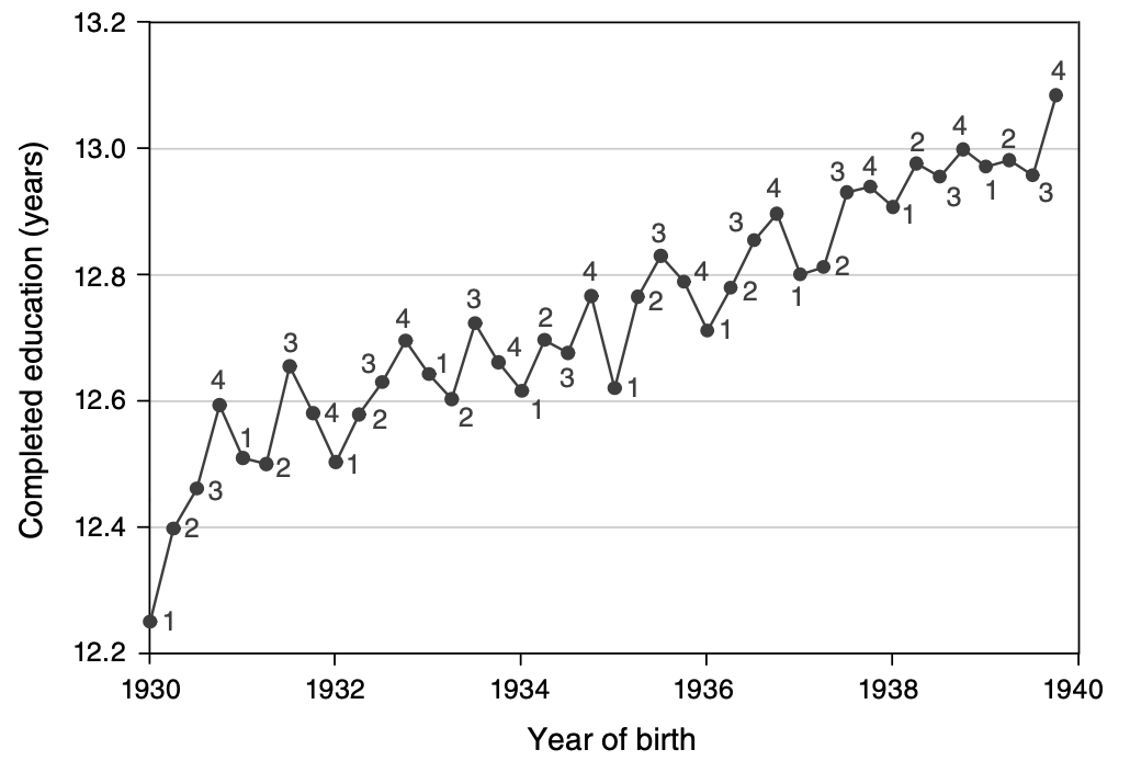
Angrist and Krueger (1991)
Compulsory schooling laws: exogenous variation by quarter of birth
Instrumental variable approach
Local Average Treatment Effect (LATE)
\[ \begin{align} \ln W_{icq} &= \beta X_i + \rho E_i + \sum_c 1\{YOB_i = c\}\xi_c + \mu_i \\ E_{icq} &= \pi X_i + \sum_c 1\{YOB_i = c\}\delta_c + \sum_c\sum_q1\{YOB_i = c\} 1\{QOB_i = q\}\theta_{qc} + \epsilon_i \end{align} \]
Causal estimates of returns to schooling
Angrist and Krueger (1991)
IV estimates of returns to education \(\rho\)
Issues:
Instrument is weak (IV estimates are inflated)
Who are the compliers? Endogeneity? External validity?
Causal estimates of returns to schooling
Some other IV approaches
| Instrument | Estimated \(\rho\) | |
|---|---|---|
| Card (1993) | Proximity to college | 0.132 (0.055) |
| Cameron and Taber (2004) | Proximity to college | 0.228 (0.109) |
| Cameron and Taber (2004) | Earnings in local labour market | 0.057 (0.115) |
| Kane and Rouse (1995) | College tuition fees | 0.116 (0.045) |
| Oreopoulos (2007) | Changes in compulsory schooling laws | 0.133 (0.0118) US 0.084 (0.0267) Canada 0.158 (0.0491) UK |
Causal estimates of returns to schooling
Twin studies
\[ \begin{align} \ln w_{ij} &= \alpha + \rho s_{ij} + A_j + \varepsilon_{ij}, ~\forall i \in \{1, 2\} \\ \Delta \ln w_j &= \rho \Delta s_j + \Delta \varepsilon_j \end{align} \]
| Estimated \(\rho\) | |
|---|---|
| Ashenfelter and Rouse (1998) | 0.088 (0.025) |
| Oreopoulos and Salvanes (2011) | 0.0476 (0.0026) |
Causal estimates of returns to schooling
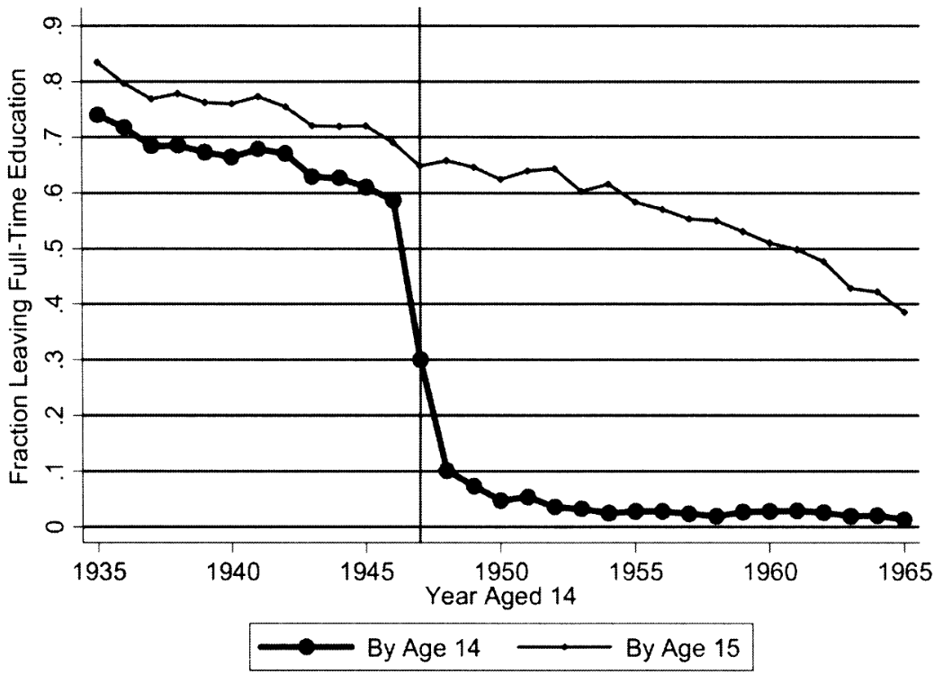
Regression discontinuity design: Oreopoulos (2006)
UK 1947: raised min school leaving age (ROSLA) from 14 to 15
Compare similar people just before and after policy change
Estimated \(\rho\) = 0.069 (0.040)
Second reform in 1972: min SLA \(\uparrow\) from 15 to 16
Small (or zero) return (Dickson and Smith 2011)
Causal estimates of returns to schooling
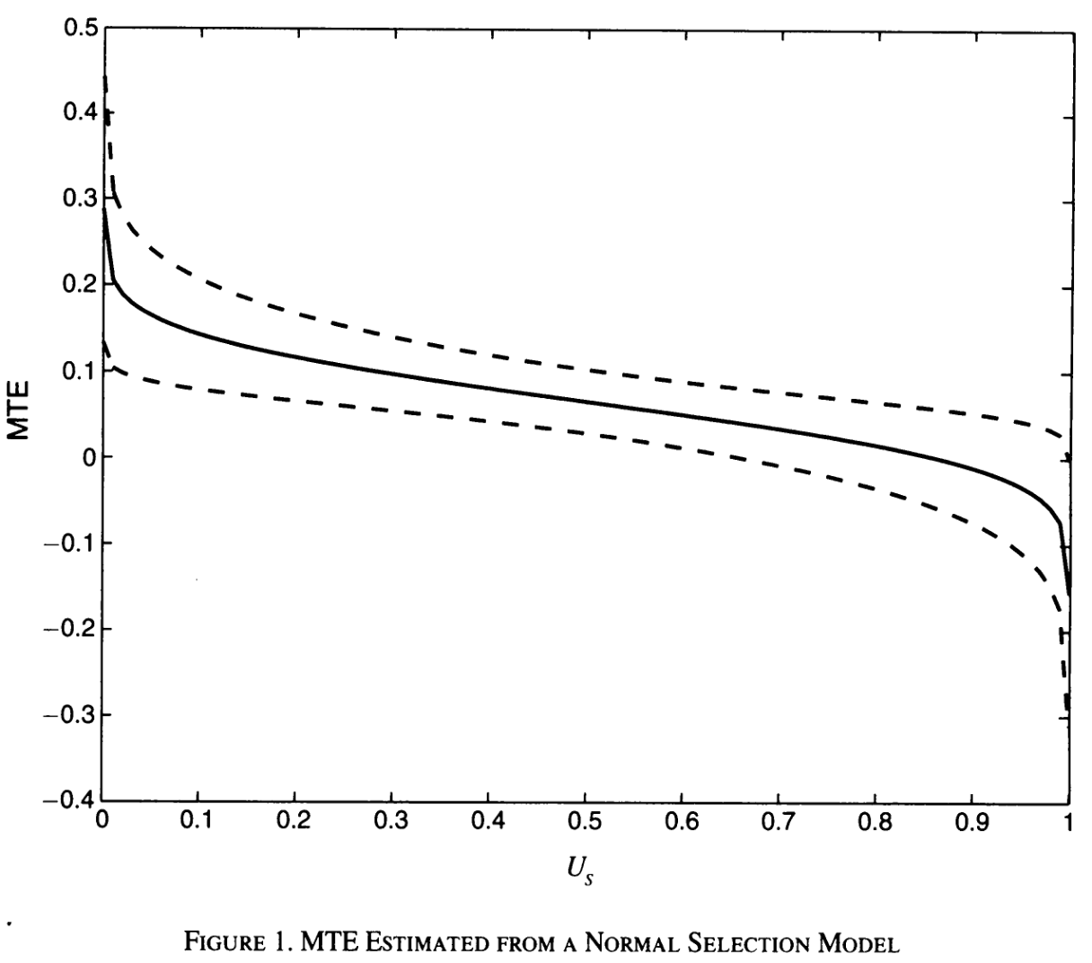
Carneiro, Heckman, and Vytlacil (2011)
- Many papers estimate sizable returns to schooling
- Average dropout rate in OECD 17% in 2020
- Heterogeneity in returns to schooling
Role of individual characteristics? E.g., patience (Cadena and Keys 2015)
Causal estimates of returns to schooling
Productivity or signalling?
Hard question to answer
Productivity
- [No] upstream effects of ROSLA on qualifications (Chevalier et al. 2004)
- Student riots, \(\uparrow\) passes, \(\uparrow\) higher edu, \(\uparrow\) wages (Maurin and McNally 2008)
- RDD of just passing/failing high school exam: no effect (Clark and Martorell 2014)
Signalling
- Employer learning: 30% of returns due to signalling (Aryal, Bhuller, and Lange 2022)
- Positive effect of degree classes (Feng and Graetz 2017)
Summary
Education is a human capital investment
Models describing the investment decisions treat education as productivity enhancing and/or signalling device
Empirical estimates suggest sizable wage returns to a year of schooling
However, still a lot of debate about causality, heterogeneity and interpretation
Next: Education Quality
References
Angrist, Joshua D., and Alan B. Krueger. 1991. “Does Compulsory School Attendance Affect Schooling and Earnings?*.” The Quarterly Journal of Economics 106 (4): 979–1014. https://doi.org/10.2307/2937954.
Aryal, Gaurab, Manudeep Bhuller, and Fabian Lange. 2022. “Signaling and Employer Learning with Instruments.” American Economic Review 112 (5): 1669–1702. https://doi.org/10.1257/aer.20200146.
Ashenfelter, Orley, and Cecilia Rouse. 1998. “Income, Schooling, and Ability: Evidence from a New Sample of Identical Twins.” The Quarterly Journal of Economics 113 (1): 253–84. https://www.jstor.org/stable/2586991.
Ben-Porath, Yoram. 1967. “The Production of Human Capital and the Life Cycle of Earnings.” Journal of Political Economy 75 (4): 352–65. https://www.jstor.org/stable/1828596.
Cadena, Brian C., and Benjamin J. Keys. 2015. “Human Capital and the Lifetime Costs of Impatience.” American Economic Journal: Economic Policy 7 (3): 126–53. https://doi.org/10.1257/pol.20130081.
Cahuc, Pierre. 2004. Labor Economics. Cambridge (Mass.): MIT Press.
Cameron, Stephen V., and Christopher Taber. 2004. “Estimation of Educational Borrowing Constraints Using Returns to Schooling.” Journal of Political Economy 112 (1): 132–82. https://doi.org/10.1086/379937.
Card, David. 1993. “Using Geographic Variation in College Proximity to Estimate the Return to Schooling.” NBER Working Paper. Cambridge, MA. October 1993. https://doi.org/10.3386/w4483.
———. 1999. “The Causal Effect of Education on Earnings.” In Handbook of Labor Economics, 3:1801–63. Elsevier. https://doi.org/10.1016/S1573-4463(99)03011-4.
Carneiro, Pedro, James J. Heckman, and Edward J. Vytlacil. 2011. “Estimating Marginal Returns to Education.” The American Economic Review 101 (6): 2754–81. https://www.jstor.org/stable/23045657.
Chevalier, Arnaud, Colm Harmon, Ian Walker, and Yu Zhu. 2004. “Does Education Raise Productivity, or Just Reflect It?” The Economic Journal 114 (499): F499–517. https://www.jstor.org/stable/3590169.
Clark, Damon, and Paco Martorell. 2014. “The Signaling Value of a High School Diploma.” Journal of Political Economy 122 (2): 282–318. https://doi.org/10.1086/675238.
Cunha, Flavio, and James Heckman. 2007. “The Technology of Skill Formation.” American Economic Review 97 (2): 31–47. https://doi.org/10.1257/aer.97.2.31.
Dickson, Matt, and Sarah Smith. 2011. “What Determines the Return to Education: An Extra Year or a Hurdle Cleared?” Economics of Education Review, Special Issue: Economic Returns to Education, 30 (6): 1167–76. https://doi.org/10.1016/j.econedurev.2011.05.004.
Feng, Andy, and Georg Graetz. 2017. “A Question of Degree: The Effects of Degree Class on Labor Market Outcomes.” Economics of Education Review 61 (December): 140–61. https://doi.org/10.1016/j.econedurev.2017.07.003.
Heckman, James, Jora Stixrud, and Sergio Urzua. 2006. “The Effects of Cognitive and Noncognitive Abilities on Labor Market Outcomes and Social Behavior.” Journal of Labor Economics 24 (3): 411–82.
Kane, Thomas J., and Cecilia Elena Rouse. 1995. “Labor-Market Returns to Two- and Four-Year College.” The American Economic Review 85 (3): 600–614. https://www.jstor.org/stable/2118190.
Maurin, Eric, and Sandra McNally. 2008. “Vive La Révolution! Long‐Term Educational Returns of 1968 to the Angry Students.” Journal of Labor Economics 26 (1): 1–33. https://doi.org/10.1086/522071.
Mincer, Jacob. 1958. “Investment in Human Capital and Personal Income Distribution.” Journal of Political Economy 66 (4): 281–302. https://www.jstor.org/stable/1827422.
Mincer, Jacob A. 1974. Schooling, Experience, and Earnings. Book. National Bureau of Economic Research. https://www.nber.org/books-and-chapters/schooling-experience-and-earnings.
Oreopoulos, Philip. 2006. “Estimating Average and Local Average Treatment Effects of Education When Compulsory Schooling Laws Really Matter.” American Economic Review 96 (1): 152–75. https://doi.org/10.1257/000282806776157641.
———. 2007. “Do Dropouts Drop Out Too Soon? Wealth, Health and Happiness from Compulsory Schooling.” Journal of Public Economics 91 (11-12): 2213–29. https://doi.org/10.1016/j.jpubeco.2007.02.002.
Oreopoulos, Philip, and Kjell G Salvanes. 2011. “Priceless: The Nonpecuniary Benefits of Schooling.” Journal of Economic Perspectives 25 (1): 159–84. https://doi.org/10.1257/jep.25.1.159.