Bell, Brian, and Stephen Machin. 2018.
“Minimum Wages and Firm Value.” Journal of Labor Economics 36 (1): 159–95.
https://doi.org/10.1086/693870.
Brown, Charles. 1999.
“Chapter 32 Minimum Wages, Employment, and the Distribution of Income.” In
Handbook of Labor Economics, 3:2101–63. Elsevier.
https://doi.org/10.1016/S1573-4463(99)30018-3.
Cahuc, Pierre. 2004. Labor Economics. Cambridge (Mass.): MIT Press.
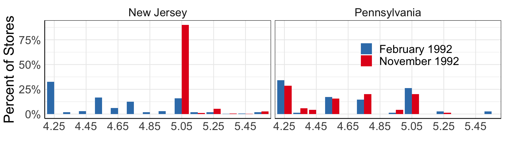
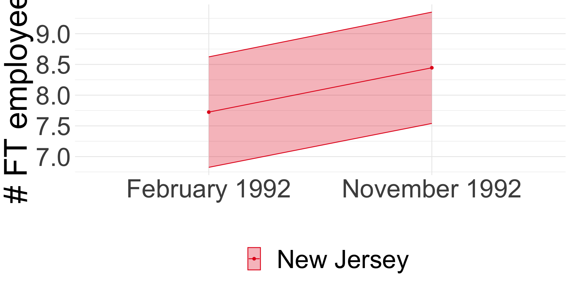
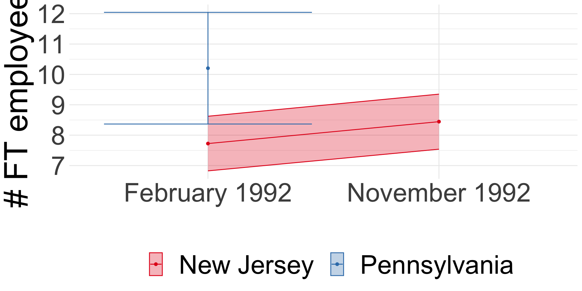
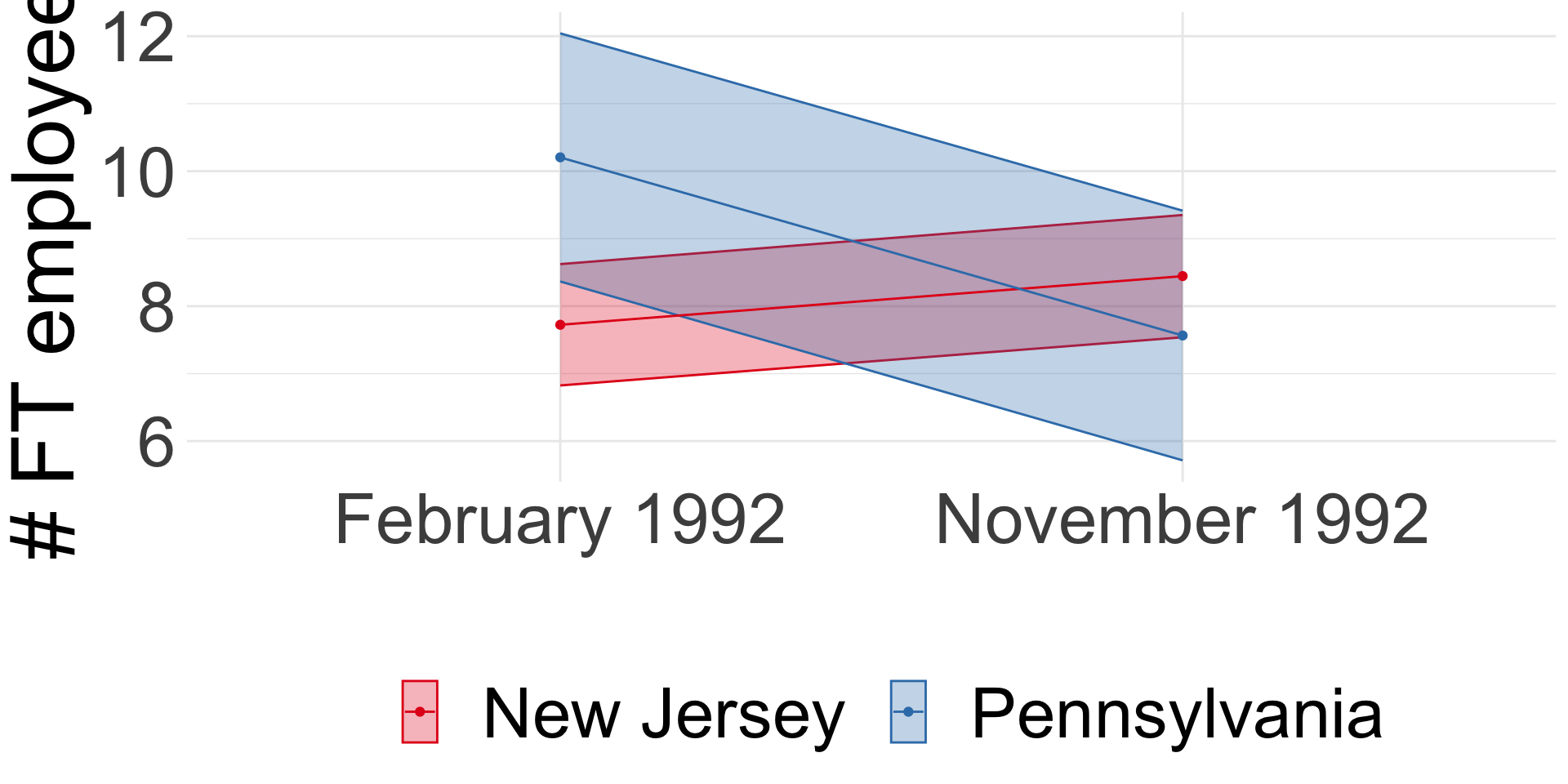
Card, David, and Alan B. Krueger. 1994.
“Minimum Wages and Employment: A Case Study of the Fast-Food Industry in New Jersey and Pennsylvania.” The American Economic Review 84 (4): 772–93.
https://www.jstor.org/stable/2118030.
Clemens, Jeffrey. 2021.
“How Do Firms Respond to Minimum Wage Increases? Understanding the Relevance of Non-Employment Margins.” Journal of Economic Perspectives 35 (1): 51–72.
https://doi.org/10.1257/jep.35.1.51.
Clemens, Jeffrey, Lisa B. Kahn, and Jonathan Meer. 2018.
“The Minimum Wage, Fringe Benefits, and Worker Welfare.” NBER Working Paper. Working
Paper Series. May 2018.
https://doi.org/10.3386/w24635.
Clemens, Jeffrey, and Michael R. Strain. 2020.
“Implications of Schedule Irregularity as a Minimum Wage Response Margin.” Applied Economics Letters 27 (20): 1691–94.
https://doi.org/10.1080/13504851.2020.1713978.
Coviello, Decio, Erika Deserranno, and Nicola Persico. 2022.
“Minimum Wage and Individual Worker Productivity: Evidence from a Large US Retailer.” Journal of Political Economy 130 (9): 2315–60.
https://doi.org/10.1086/720397.
Draca, Mirko, Stephen Machin, and John Van Reenen. 2011.
“Minimum Wages and Firm Profitability.” American Economic Journal: Applied Economics 3 (1): 129–51.
https://doi.org/10.1257/app.3.1.129.
Dustmann, Christian, Attila Lindner, Uta Schönberg, Matthias Umkehrer, and Philipp vom Berge. 2022.
“Reallocation Effects of the Minimum Wage*.” The Quarterly Journal of Economics 137 (1): 267–328.
https://doi.org/10.1093/qje/qjab028.
Hamermesh, Daniel S. 1996. Labor Demand. Princeton University Press.
Houseman, Susan N, and Katharine G Abraham. 1993.
“Labor Adjustment Under Different Institutional Structures: A Case Study of Germany and the United States.” NBER Working Paper 4548. Cambridge, MA. October 1993.
https://www.nber.org/system/files/working_papers/w4548/w4548.pdf.
Jardim, Ekaterina, Mark C. Long, Robert Plotnick, Emma van Inwegen, Jacob Vigdor, and Hilary Wething. 2022.
“Minimum-Wage Increases and Low-Wage Employment: Evidence from Seattle.” American Economic Journal: Economic Policy 14 (2): 263–314.
https://doi.org/10.1257/pol.20180578.
Ku, Hyejin. 2022.
“Does Minimum Wage Increase Labor Productivity? Evidence from Piece Rate Workers.” Journal of Labor Economics 40 (2): 325–59.
https://doi.org/10.1086/716347.
Leung, Justin H. 2021.
“Minimum Wage and Real Wage Inequality: Evidence from Pass-Through to Retail Prices.” The Review of Economics and Statistics 103 (4): 754–69.
https://doi.org/10.1162/rest_a_00915.
Luca, Dara Lee, and Michael Luca. 2019.
“Survival of the Fittest: The Impact of the Minimum Wage on Firm Exit.” NBER Working Paper. Working
Paper Series. May 2019.
https://doi.org/10.3386/w25806.
Nickell, S. J. 1986.
“Chapter 9 Dynamic Models of Labour Demand.” In
Handbook of Labor Economics, 1:473–522. Elsevier.
https://doi.org/10.1016/S1573-4463(86)01012-X.
Reich, Michael, Sylvia Allegretto, and Anna Goddy. 2017.
“Seattle’s Minimum Wage Experience 2015-16.” SSRN Electronic Journal.
https://doi.org/10.2139/ssrn.3043388.
Renkin, Tobias, Claire Montialoux, and Michael Siegenthaler. 2022.
“The Pass-Through of Minimum Wages into U.S. Retail Prices: Evidence from Supermarket Scanner Data.” The Review of Economics and Statistics 104 (5): 890–908.
https://doi.org/10.1162/rest_a_00981.