3. Labour Demand
KAT.TAL.322 Advanced Course in Labour Economics
Nurfatima Jandarova
March 13, 2024
Labour demand
Firm decisions about how much labour to hire.
Static model
Static model
Single factor input
Production function Y=F(L) where F′>0 and F′′<0
maxLPF(L)−WL
FOC: F′(L)=WP
Downward-sloping labour demand ∂L∂W=1PF′′(L)<0
Static model
Two factor inputs: conditional factor demand
Cost minimization problem
minL,KC(L,K)=WL+RK s.t. F(L,K)=ˉY
Conditional demand functions ˉK(W,R,Y) and ˉL(W,R,Y)
FL(ˉL,ˉK)FK(ˉL,ˉK)=WRandF(ˉL,ˉK)=ˉY
Static model
Two factor inputs: conditional demand elasticities
Own-price elasticities: ηLW=∂lnˉL∂lnW<0, ηKR=∂lnˉK∂lnR<0
Cross-price elasticities: ηLR=∂lnˉL∂lnR>0 and ηKW=∂lnˉK∂lnW>0
Elasticity of substitution σ=∂ln(KL)∂ln(WR)>0
It is also possible to show that
ηLR=σ(1−s)andηLW=−σ(1−s)
where s=WLC is labour share in total cost
Static model
Two factor inputs: unconditional factor demand
maxYPY−C(W,R,Y)
Solution: P=CY(W,R,Y∗),L∗=ˉL(W,R,Y∗),K∗=ˉK(W,R,Y∗)
Total elasticities decomposed into substitution and scale effects:
εLW=ηLW+ηLYεYW<0
εLR=ηLR+ηLYεYR≶0
Estimations of static model
Empirical strategy
Shephard’s lemma: specify cost function and back out labour demand
Example: translog cost function with n inputs
lnC=a0+n∑i=1ailnWi+12n∑i=1n∑j=1aijlnWilnWj+1θlnY
⇒si=ai+n∑j=1aijlnWj
Estimate parameters ai,aij and calculate implied elasticities.
Estimations of static model
Main issues
Endogeneity
General equilibrium
Definitions of variables
Estimations of static model
Review by Hamermesh (1996) concludes that −ηLW∈[0.15,0.75].
If ηLW=−0.30 and given that s≈0.7,
σ=−ηLW1−s≈1
consistent with the Cobb-Douglas production function.
The review also suggests −εLW≈1⇒ large scale effect.
Dynamic model
Dynamic model
Adjustment costs
Quadratic cost: C(ΔLt)=b(ΔLt−a)2
Assymmetric convex costs: C(ΔLt)=−1+eaΔLt−aΔLt+b2(ΔLt)2
Linear cost: C(ΔLt)={chΔLtif ΔLt≥0−cfΔLtif ΔLt≤0
Fixed cost
Dynamic model
Quadratic adjustment cost
Continuous time ⇒ΔLt=˙Lt=dLtdt
Π0=∫∞0Πtdt=∫∞0[F(Lt)−WtLt−b2˙L2t]e−rtdt
Euler equation: ∂Πt∂L=ddt(∂Πt∂˙Lt)⇒b¨Lt−rb˙Lt+F′(Lt)−Wt=0
Dynamic model
Quadratic adjustment cost
Optimal path: ˙Lt=γ[L∗−Lt] where γ is decreasing in b.
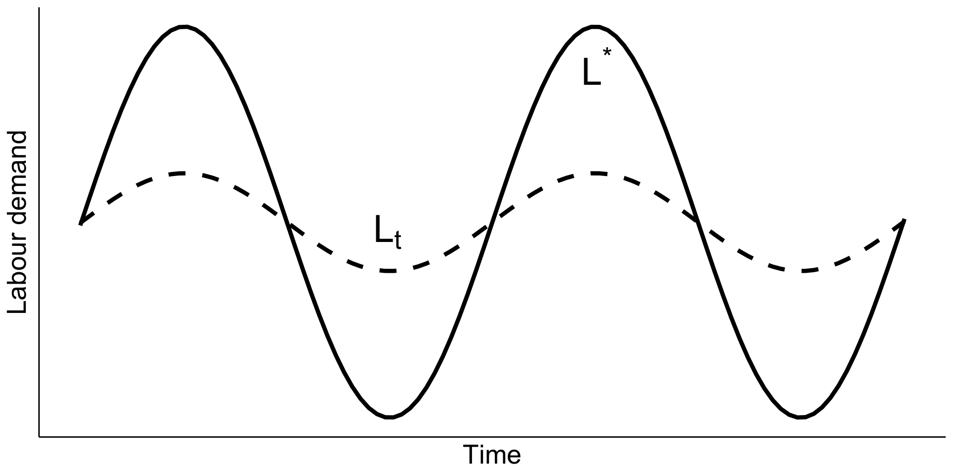
Figure 9.6 Optimal employment over a cycle (Nickell 1986)
Dynamic model
Linear adjustment cost
Π0=∫∞0[F(Lt)−WtLt−C(˙Lt)]e−rtdt
where C(˙Lt)={ch˙Ltif ˙Lt≥0−cf˙Ltif ˙Lt≤0
Optimal labour demand path is derived from
{F′(Lt)=Wt+rchif ˙Lt≥0F′(Lt)=Wt−rcfif ˙Lt<0
Dynamic model
Linear adjustment cost
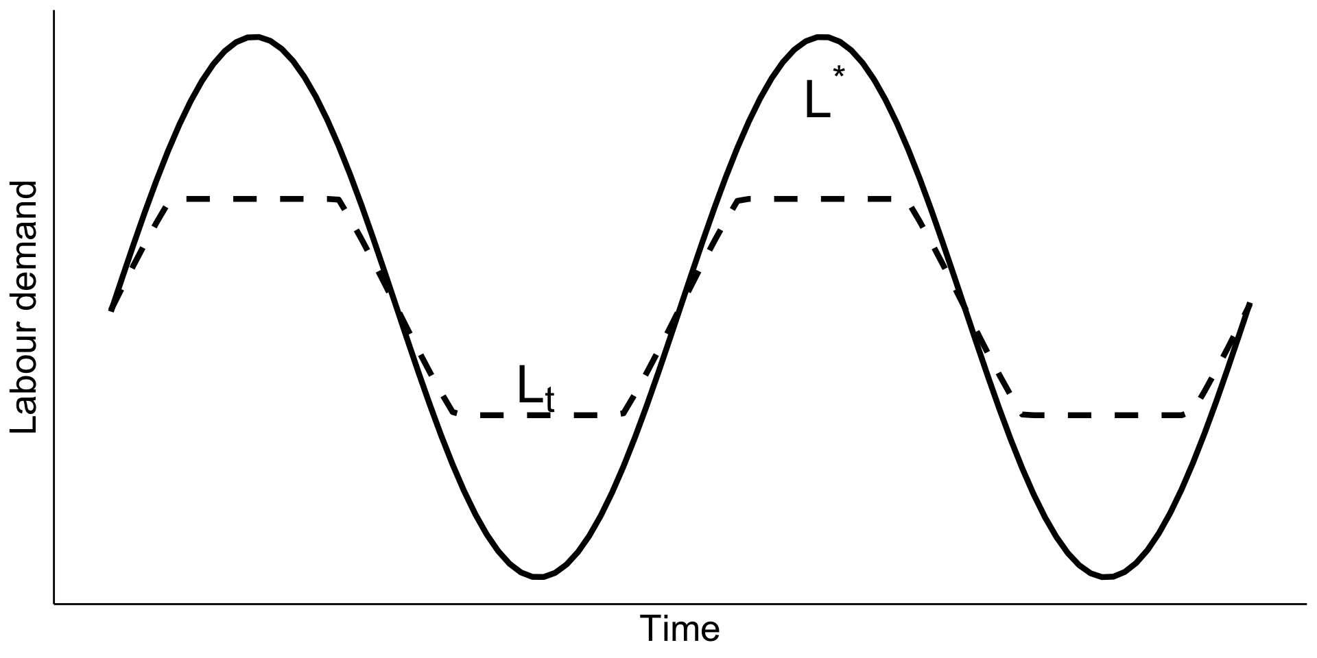
Figure 9.10 Optimal employment over the cycle (Nickell 1986)
Estimations of dynamic model
Empirical strategy for adjustment cost specification
Quadratic adjustment cost
Assume linear quadratic production function
Estimate Lit=λLi,t−1+Xitβ+μi+εit
- accounting for correlation between Li,t−1 and μi+εit
Other adjustment costs and production functions
Estimate Euler equation directly
Current employment Lt depends on past and future variables
Appropriate econometric methods (Hamilton 1994 book)
Estimations of dynamic model
Some key results
Adjustments happen fast (1-2 quarters) (Hamermesh 1996, chap. 7)
Dynamic substitutes: utilization of capital increases with Lt−L∗
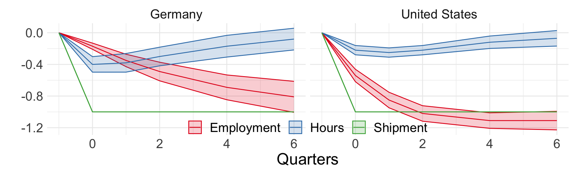
Hours of work are adjusted faster than number of workers
![]()
Figure 1 from Houseman and Abraham (1993) (adjustment to demand shocks)
Minimum wages and employment
Minimum wage and employment
What do the models we have considered so far predict?
lower labour demand (both compensated and uncompensated)
(maybe) higher labour supply
Any “problems” with these conclusions?
Typically not supported by empirical evidence!
Minimum wage and employment
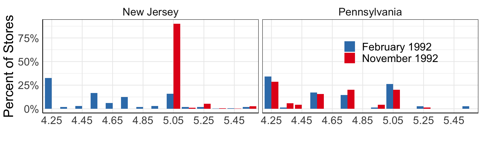
Card and Krueger (1994)
On April 1, 1992 minimum wage in New Jersey ↑ from $4.25 to $5.05.
It stayed at $4.25 in Pennsylvania.
It stayed at $4.25 in Pennsylvania.
Minimum wage and employment
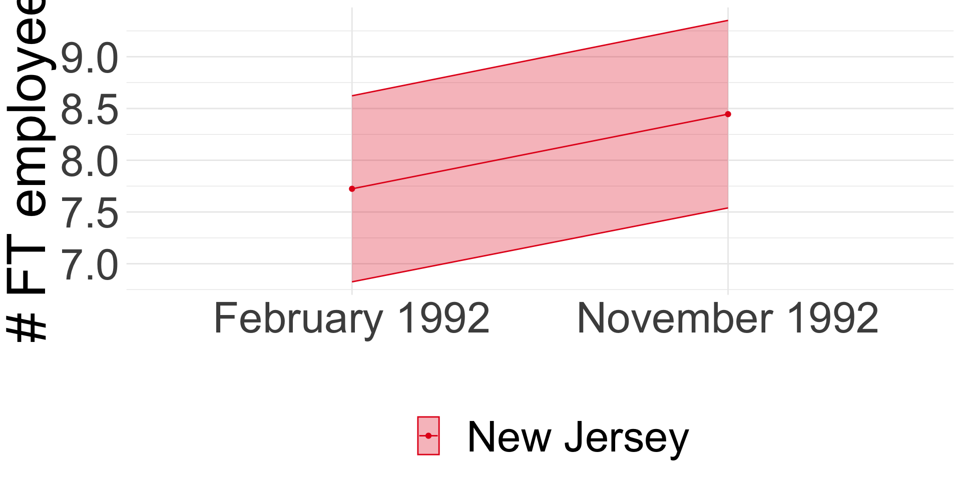
Card and Krueger (1994): Difference-in-differences
- Compare before and after:
ENJt1−ENJt0 = 0.59 (se = 0.54)
Minimum wage and employment
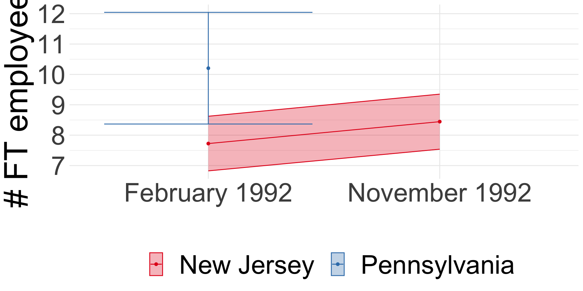
Card and Krueger (1994): Difference-in-differences
- Compare before and after:
ENJt1−ENJt0 = 0.59 (se = 0.54) - Compare NJ and PA:
ENJt−EPAt = -2.89 (se = 1.44)
Minimum wage and employment
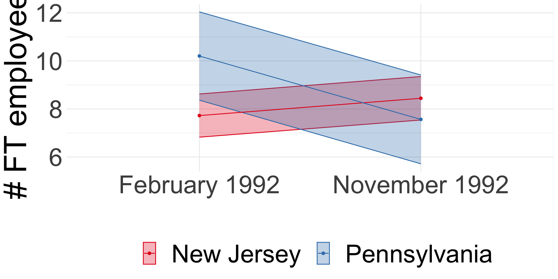
Card and Krueger (1994): Difference-in-differences
- Compare before and after:
ENJt1−ENJt0 = 0.59 (se = 0.54) - Compare NJ and PA:
ENJt−EPAt = -2.89 (se = 1.44) - Diff-in-diff:
(ENJt1−ENJt0)−(EPAt1−EPAt0) = 2.75 (se = 1.34)
Minimum wage and employment
Jardim et al. (2022)
Seattle ↑ min wage from $9.47 up to
- $11 in April 2015
- $13 in January 2016
Causal design:
- synthetic control: weighted average of other counties that match pre-Seattle
- nearest neighbour matching: find “closest” worker outside of Seattle matching treated worker in Seattle
Minimum wage and employment
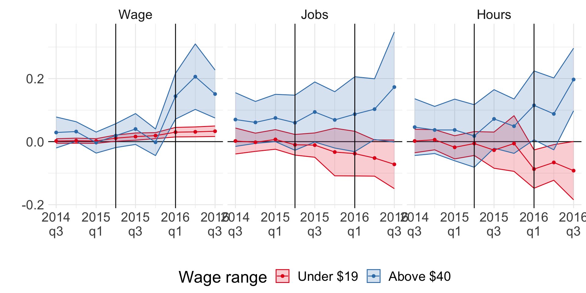
Jardim et al. (2022): synthetic control
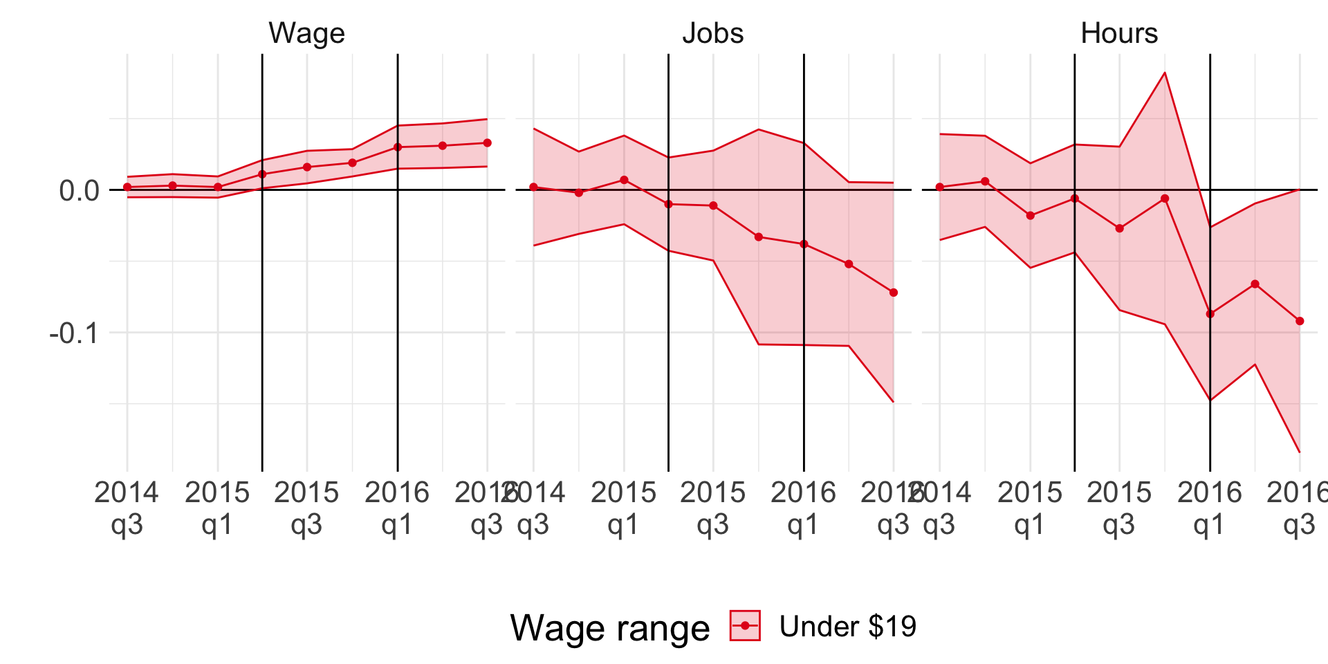
Minimum wage and employment
Jardim et al. (2022): synthetic control
Minimum wage and employment
Jardim et al. (2022)
- Negative effect on hours worked stronger than on employment
- Experienced workers are better off
However,
- Potentially cascading effect
- Excluded large low-wage employers (like McDonald’s) (monopsony)
Reich, Allegretto, and Goddy (2017)
same policy + synthetic control = no change in employment
Minimum wage and employment
Monopsony
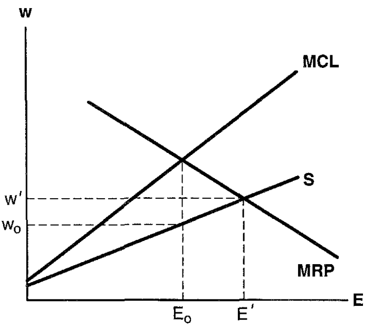
Source: Figure 3 from Brown (1999)
Minimum wage and other margins
Review in Clemens (2021)
- Price pass-through (Leung 2021; Renkin, Montialoux, and Siegenthaler 2022)
- Non-wage labour cost (Clemens, Kahn, and Meer 2018)
- Flexibility (theoretical Clemens and Strain 2020)
- Effort (Ku 2022; Coviello, Deserranno, and Persico 2022)
- Firm profit (Draca, Machin, and Van Reenen 2011; Bell and Machin 2018)
- Firm exit (Luca and Luca 2019; Dustmann et al. 2022)
Summary
Basic static and dynamic models of labour demand
Application to minimum wage policy
- Ongoing research (little consensus)
- Clear that basic models are insufficient
- Typical frameworks: heterogeneous labour, monopsony
- Non-wage margins important and can interact with labour supply
Next: Human Capital
References
Bell, Brian, and Stephen Machin. 2018. “Minimum Wages and Firm Value.” Journal of Labor Economics 36 (1): 159–95. https://doi.org/10.1086/693870.
Brown, Charles. 1999. “Chapter 32 Minimum Wages, Employment, and the Distribution of Income.” In Handbook of Labor Economics, 3:2101–63. Elsevier. https://doi.org/10.1016/S1573-4463(99)30018-3.
Cahuc, Pierre. 2004. Labor Economics. Cambridge (Mass.): MIT Press.
Card, David, and Alan B. Krueger. 1994. “Minimum Wages and Employment: A Case Study of the Fast-Food Industry in New Jersey and Pennsylvania.” The American Economic Review 84 (4): 772–93. https://www.jstor.org/stable/2118030.
Clemens, Jeffrey. 2021. “How Do Firms Respond to Minimum Wage Increases? Understanding the Relevance of Non-Employment Margins.” Journal of Economic Perspectives 35 (1): 51–72. https://doi.org/10.1257/jep.35.1.51.
Clemens, Jeffrey, Lisa B. Kahn, and Jonathan Meer. 2018. “The Minimum Wage, Fringe Benefits, and Worker Welfare.” NBER Working Paper. Working Paper Series. May 2018. https://doi.org/10.3386/w24635.
Clemens, Jeffrey, and Michael R. Strain. 2020. “Implications of Schedule Irregularity as a Minimum Wage Response Margin.” Applied Economics Letters 27 (20): 1691–94. https://doi.org/10.1080/13504851.2020.1713978.
Coviello, Decio, Erika Deserranno, and Nicola Persico. 2022. “Minimum Wage and Individual Worker Productivity: Evidence from a Large US Retailer.” Journal of Political Economy 130 (9): 2315–60. https://doi.org/10.1086/720397.
Draca, Mirko, Stephen Machin, and John Van Reenen. 2011. “Minimum Wages and Firm Profitability.” American Economic Journal: Applied Economics 3 (1): 129–51. https://doi.org/10.1257/app.3.1.129.
Dustmann, Christian, Attila Lindner, Uta Schönberg, Matthias Umkehrer, and Philipp vom Berge. 2022. “Reallocation Effects of the Minimum Wage*.” The Quarterly Journal of Economics 137 (1): 267–328. https://doi.org/10.1093/qje/qjab028.
Hamermesh, Daniel S. 1996. Labor Demand. Princeton University Press.
Houseman, Susan N, and Katharine G Abraham. 1993. “Labor Adjustment Under Different Institutional Structures: A Case Study of Germany and the United States.” NBER Working Paper 4548. Cambridge, MA. October 1993. https://www.nber.org/system/files/working_papers/w4548/w4548.pdf.
Jardim, Ekaterina, Mark C. Long, Robert Plotnick, Emma van Inwegen, Jacob Vigdor, and Hilary Wething. 2022. “Minimum-Wage Increases and Low-Wage Employment: Evidence from Seattle.” American Economic Journal: Economic Policy 14 (2): 263–314. https://doi.org/10.1257/pol.20180578.
Ku, Hyejin. 2022. “Does Minimum Wage Increase Labor Productivity? Evidence from Piece Rate Workers.” Journal of Labor Economics 40 (2): 325–59. https://doi.org/10.1086/716347.
Leung, Justin H. 2021. “Minimum Wage and Real Wage Inequality: Evidence from Pass-Through to Retail Prices.” The Review of Economics and Statistics 103 (4): 754–69. https://doi.org/10.1162/rest_a_00915.
Luca, Dara Lee, and Michael Luca. 2019. “Survival of the Fittest: The Impact of the Minimum Wage on Firm Exit.” NBER Working Paper. Working Paper Series. May 2019. https://doi.org/10.3386/w25806.
Nickell, S. J. 1986. “Chapter 9 Dynamic Models of Labour Demand.” In Handbook of Labor Economics, 1:473–522. Elsevier. https://doi.org/10.1016/S1573-4463(86)01012-X.
Reich, Michael, Sylvia Allegretto, and Anna Goddy. 2017. “Seattle’s Minimum Wage Experience 2015-16.” SSRN Electronic Journal. https://doi.org/10.2139/ssrn.3043388.
Renkin, Tobias, Claire Montialoux, and Michael Siegenthaler. 2022. “The Pass-Through of Minimum Wages into U.S. Retail Prices: Evidence from Supermarket Scanner Data.” The Review of Economics and Statistics 104 (5): 890–908. https://doi.org/10.1162/rest_a_00981.

3. Labour Demand KAT.TAL.322 Advanced Course in Labour Economics Nurfatima Jandarova March 13, 2024