8. Technological shift and labour markets
KAT.TAL.322 Advanced Course in Labour Economics
September 17, 2025
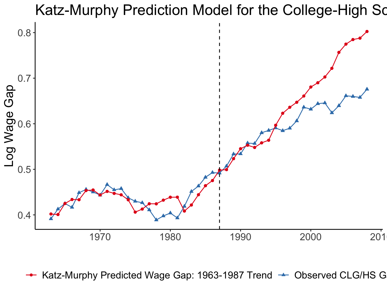
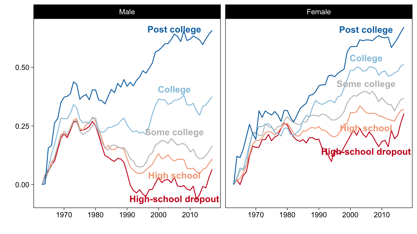
Labour market of educated workers
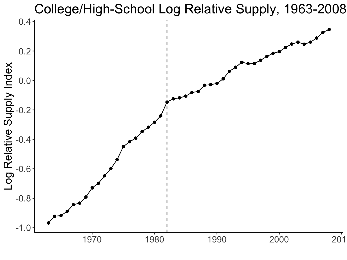
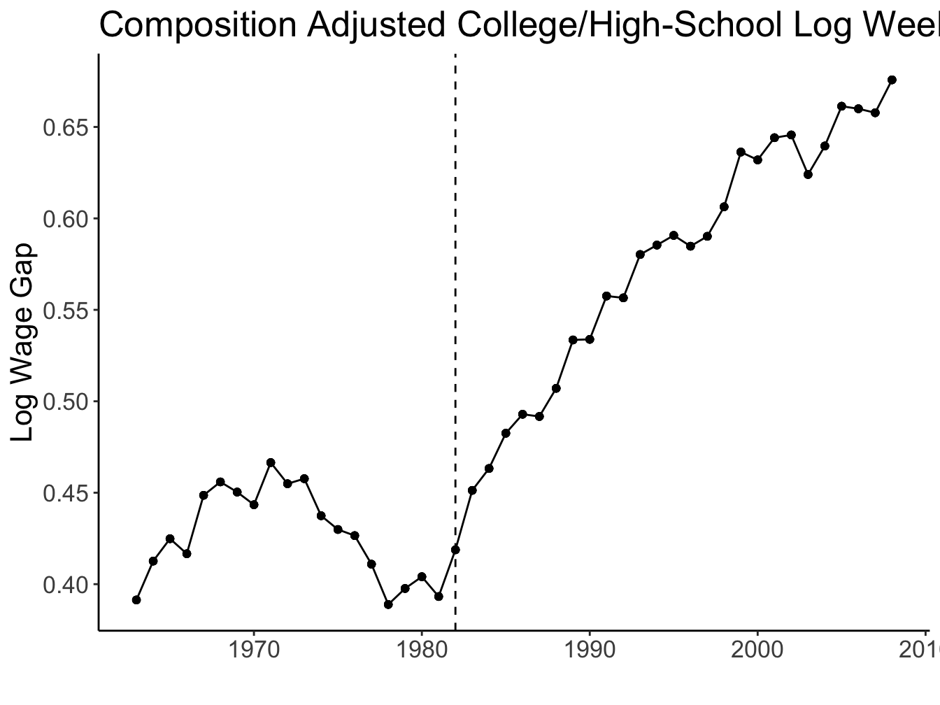
Source: Figures 1 and 2 (Acemoglu and Autor 2011)
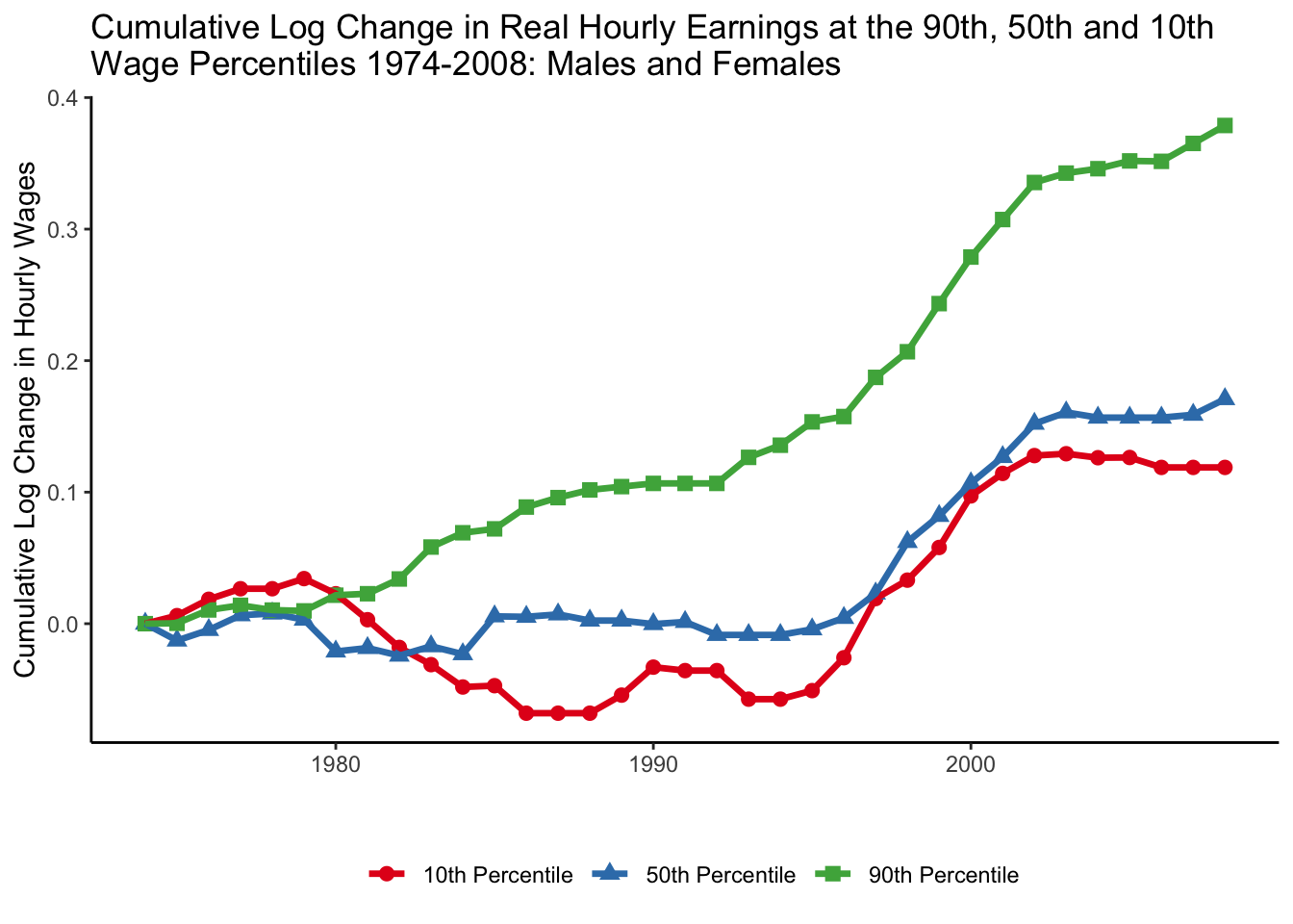
Unexplained trend: falling real wages
Source: Figure 1 (Autor 2019)
Unexplained trend: earnings polarization
Source: Figure 8 (Acemoglu and Autor 2011)
Unexplained trend: job polarization
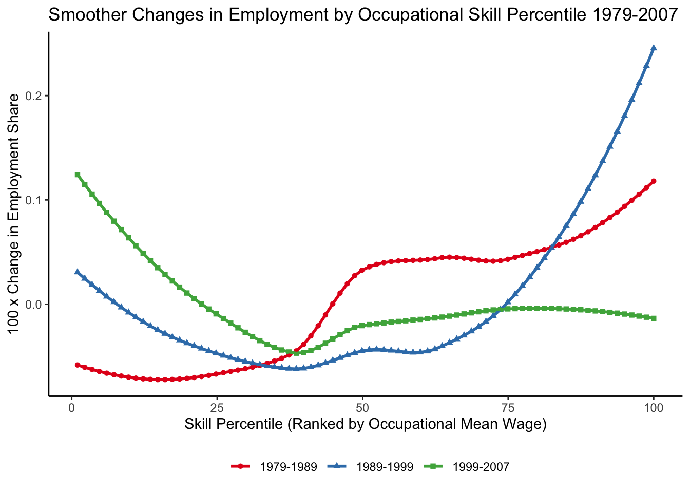
Source: Figure 10 (Acemoglu and Autor 2011)
Task-based model
Equilibrium without machines
Lemma 1
Given comparative advantage assumption, there exist \(I_L\) and \(I_H\) such that

Note that boundaries \(I_L\) and \(I_H\) are endogenous
This gives rise to the substitution of skills across tasks
Task-based model
Endogenous thresholds: no arbitrage
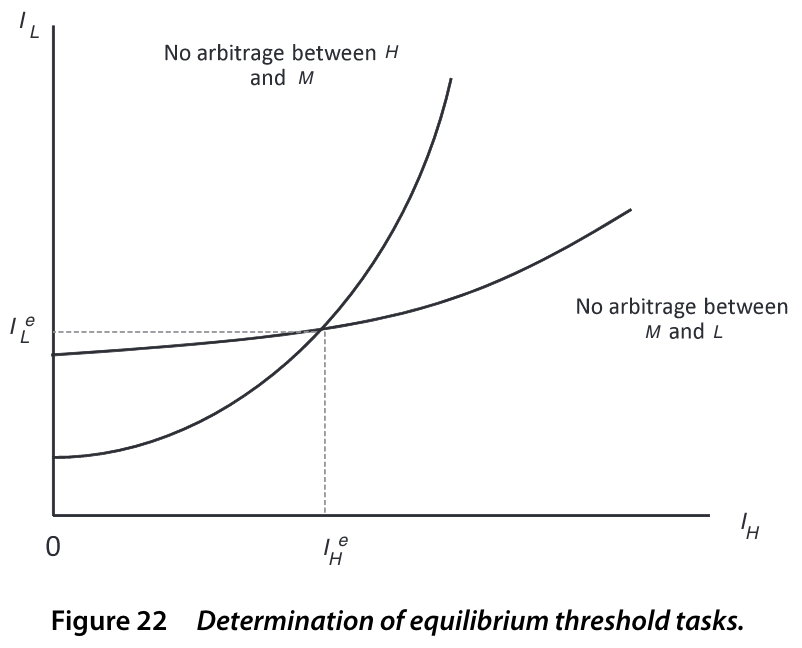
Task-based model
Comparative statics: \(\uparrow A_H\)

Source: Figure 25 (Acemoglu and Autor 2011)
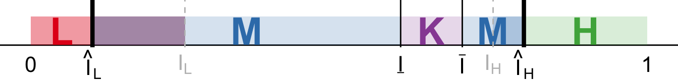
Task-based model
Task replacing technologies
Start from initial equilibrium without machines

Assume in \([\underline{I}, \bar{I}] \subset [I_L, I_H]\) machines outperform \(M\). Otherwise, \(\alpha_K(i) = 0\).

How does it change the equilibrium?
Task-based model
Task replacing technologies

Assume comparative advantage of \(H\) over \(M\) stronger than \(M\) over \(L\)
- \(w_H / w_M\) increases
- \(w_M / w_L\) decreases
- \(w_H / w_L \uparrow \color{#9a2515}{\left(\downarrow\right)}\) if \(\left|\beta^\prime_L(I_L) I_L\right| \stackrel{<}{\color{#9a2515}{>}} \left|\beta^\prime_H(I_H)(1 - I_H)\right|\)
Task-based model
Endogenous supply of skills
Each worker \(j\) is endowed with some amount of each skill \(l^j, m^j, h^j\)
Workers allocate time to each skill given
\[ \begin{align} &t_l^j + t_m^j + t_h^j \leq 1 \\ &w_L t_l^j l^j + w_M t_m^j m^j + w_H t_h^j h^j \end{align} \]
Comparative advantage: \(\frac{h^j}{m^j}\) and \(\frac{m^j}{l^j}\) are decreasing in \(j\)
Then, there exist \(J^\star\left(\frac{w_H}{w_M}\right)\) and \(J^{\star\star}\left(\frac{w_M}{w_L}\right)\)

Task-based model
Illustration in the data
Source: Table 10 (Acemoglu and Autor 2011)
Acemoglu and Restrepo (2022)
Environment
Multi-sector model with imperfect substitution between inputs
\[ \text{Task displacement}_g^\text{direct} = \sum_{i \in \mathcal{I}} \omega_g^i \frac{\omega_{gi}^R}{\omega_i^R} \left(-d \ln s_i^{L, \text{auto}}\right) \]
\(\omega_g^i\) - share of wages earned by worker group \(g\) in industry \(i\)
(exposure to industry \(i\))at \(t=0\)\(\frac{\omega_{gi}^R}{\omega_i^R}\) - specialization of group \(g\) in routine tasks \(R\) within industry \(i\) at \(t=0\)
\(-d \ln s_i^{L, \text{auto}}\) - % decline in industry \(i\)’s labour share due to automation
attribute 100% of the decline to automation
predict given industry adoption of automation technology
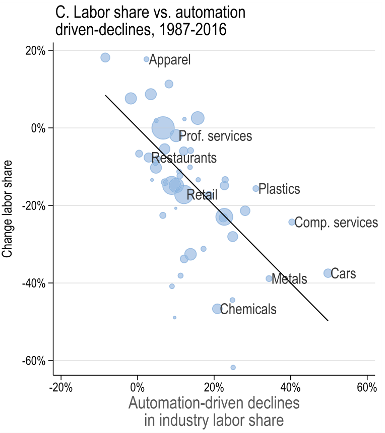
Acemoglu and Restrepo (2022)
Task displacement
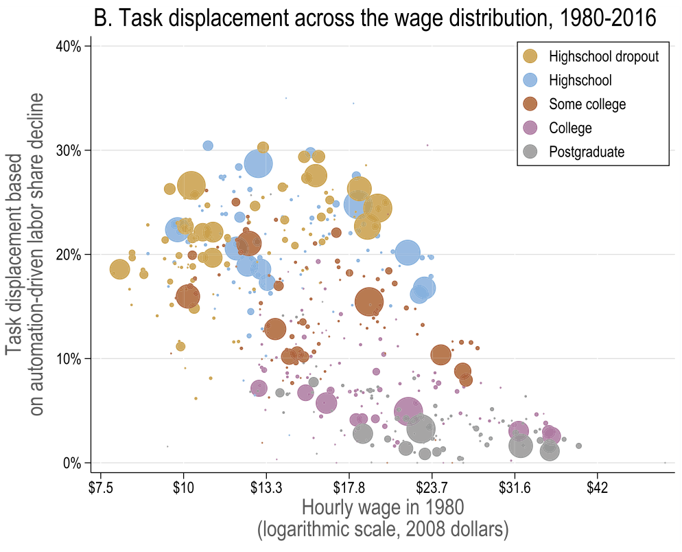
Source: Figure 5
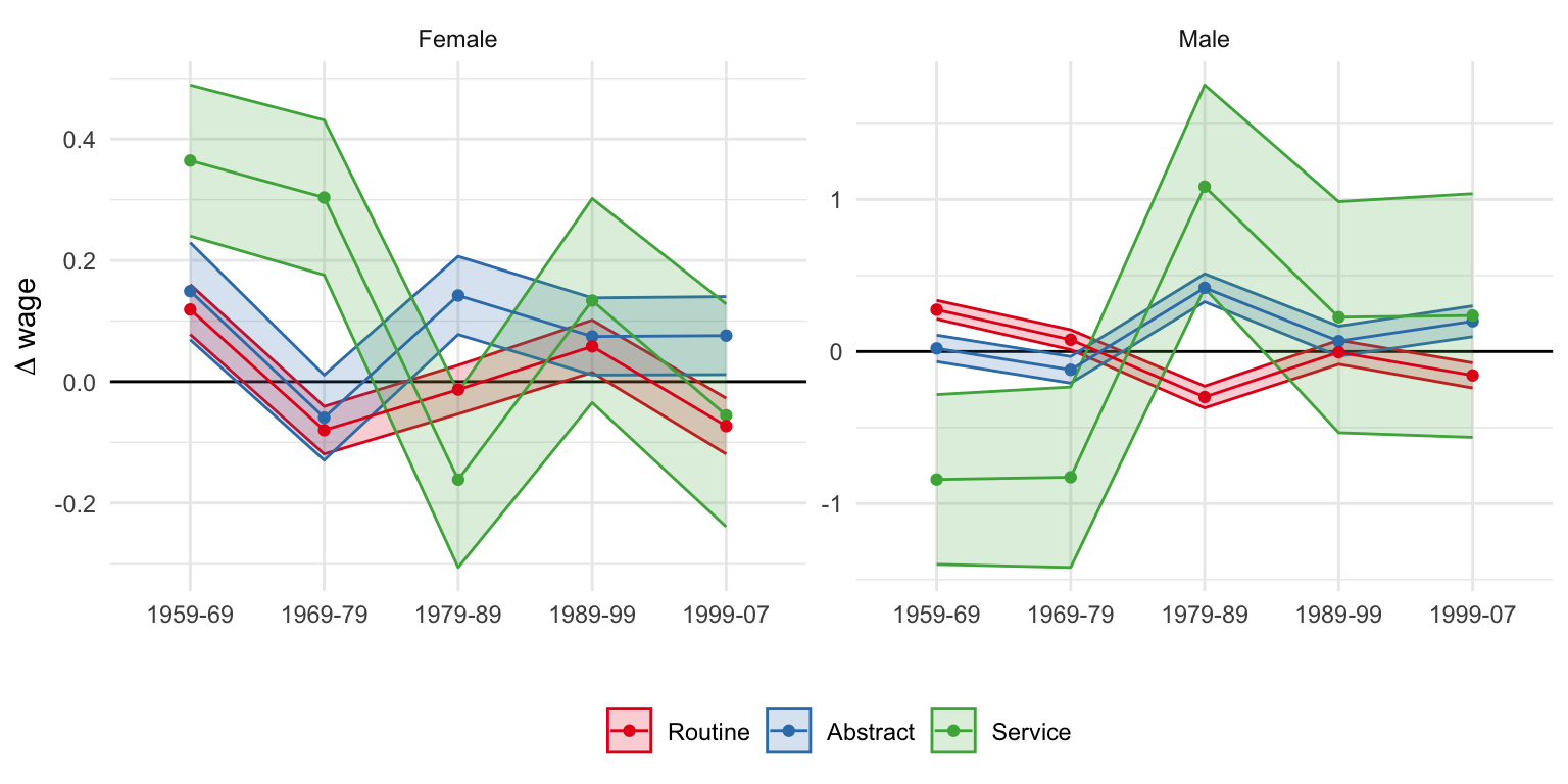
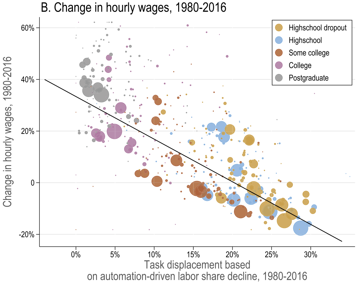
Acemoglu and Restrepo (2022)
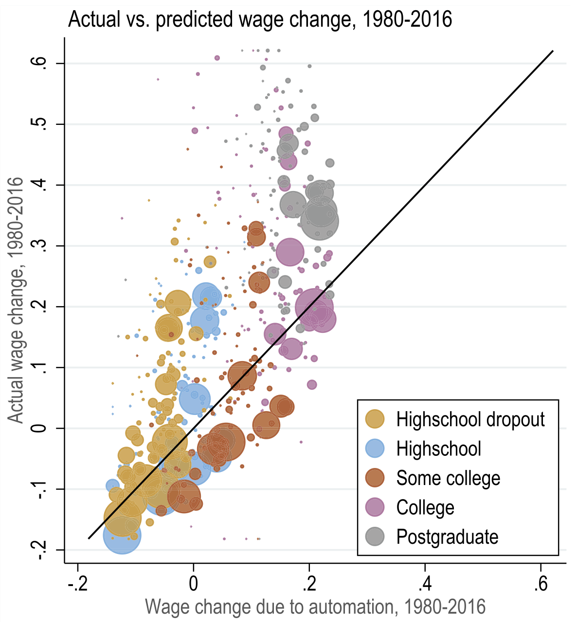
Task displacement and changes in real wages
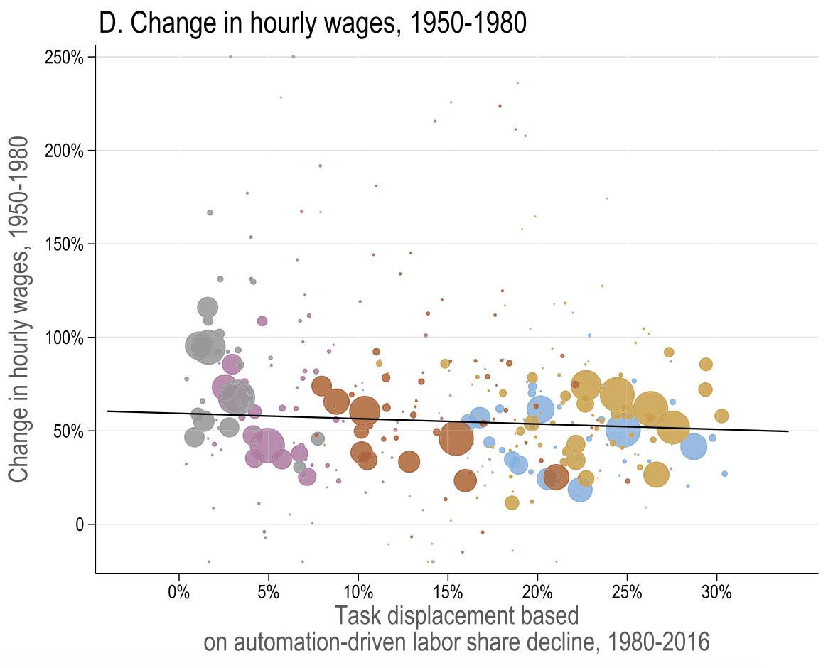
Acemoglu and Restrepo (2022)
General equilibrium results
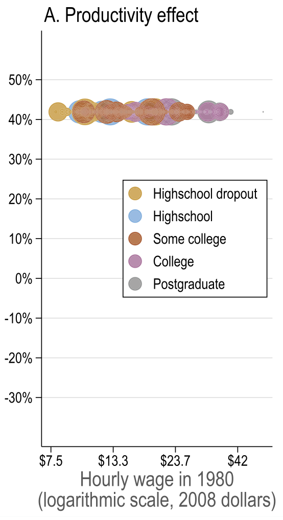
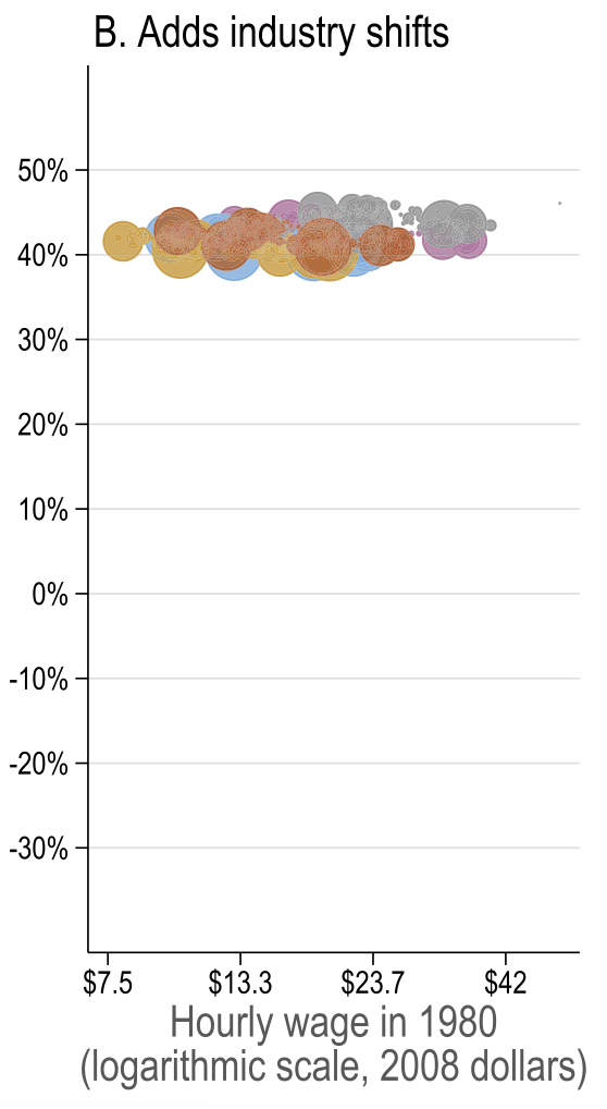
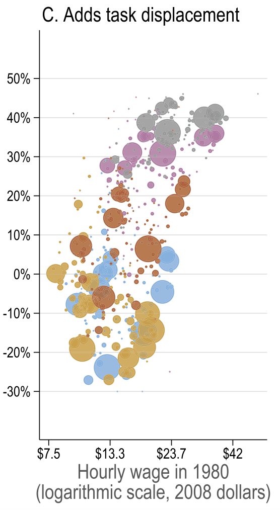
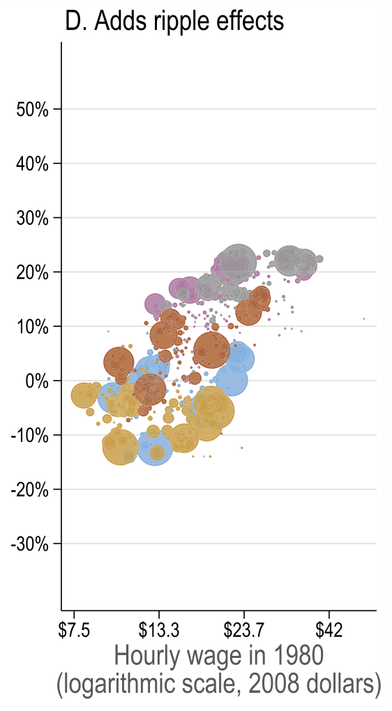
Source: Figure 7 (Acemoglu and Restrepo 2022)
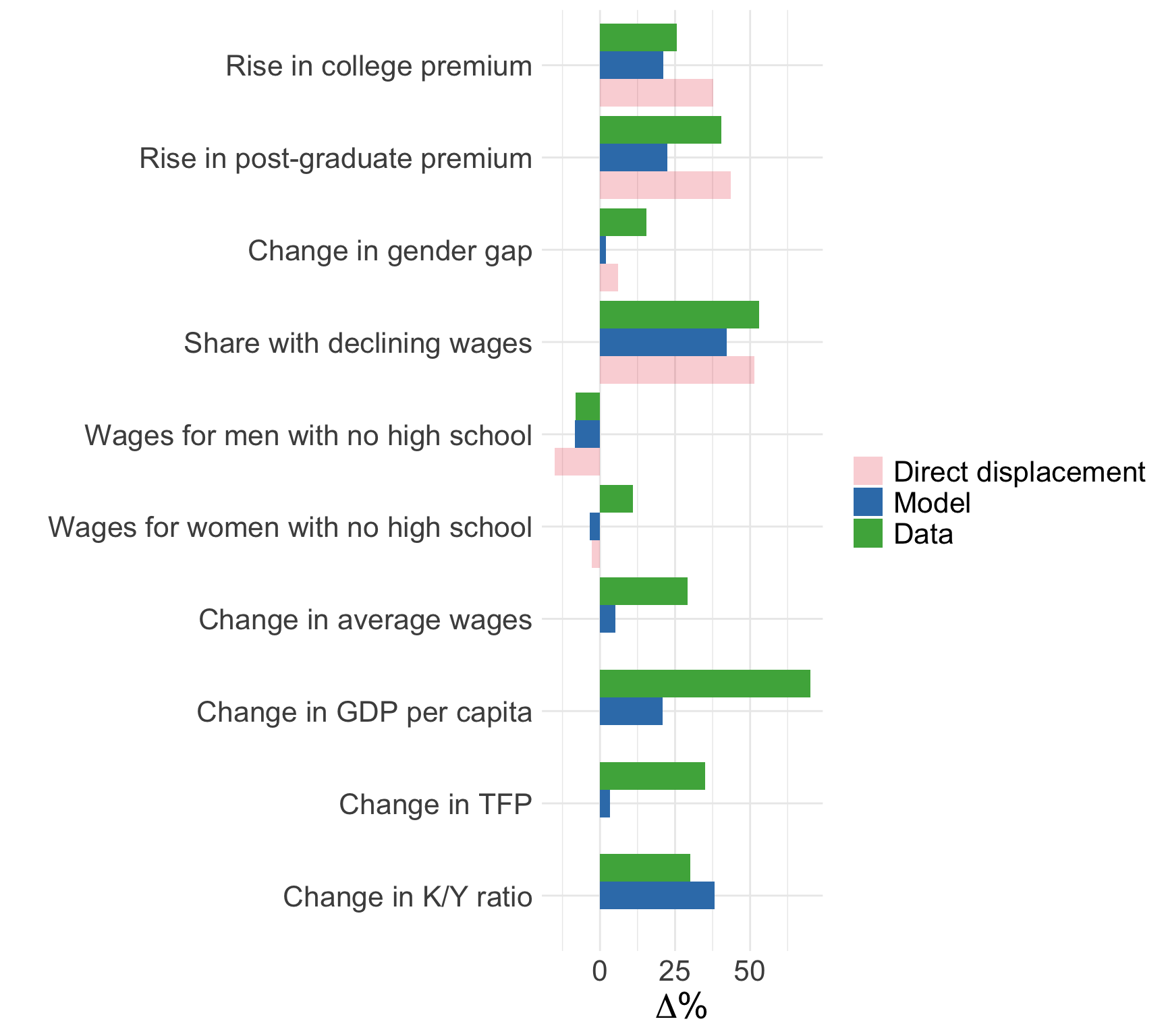
Acemoglu and Restrepo (2022)
Model fit