5. Wage setting

KAT.TAL.322 Advanced Course in Labour Economics

Nurfatima Jandarova

September 8, 2025

Today

• Stylised facts
• Perfect competition
• Imperfect competition
• Empirical evidence

• Why do wages differ between workers?
  • Compensating differentials
  • Bargaining power of firms and workers
  • Imperfect information about productivities and jobs
• Relative contributions of different sources to overall wage inequality

Stylised facts

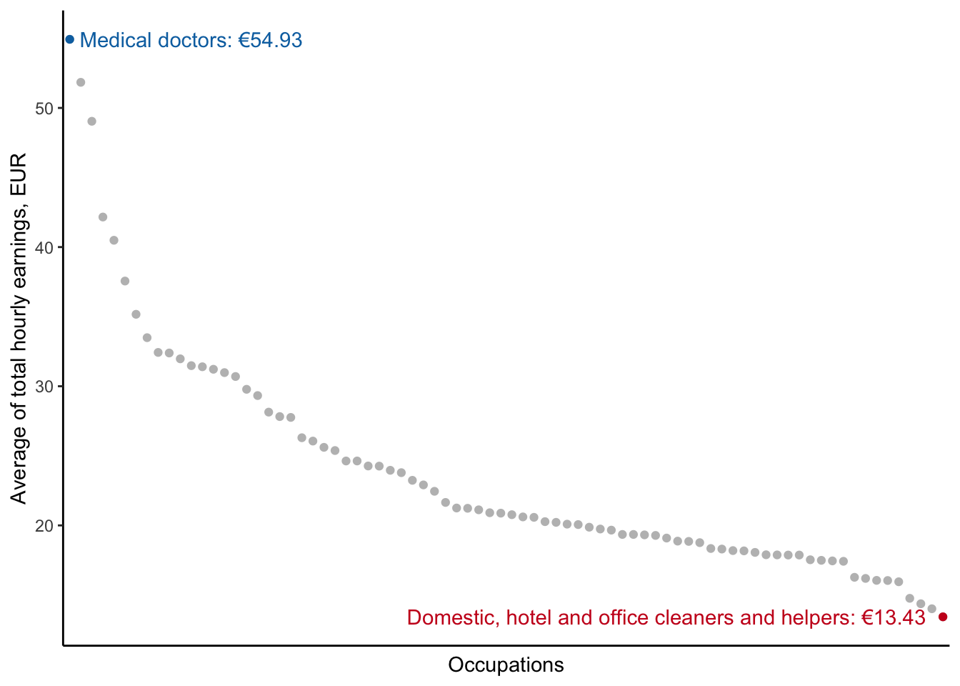
Wage dispersion

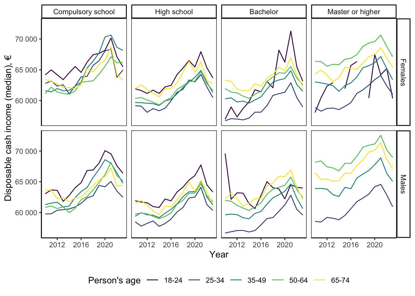
Source: Statistics Finland

The central question of today’s lecture is wage dispersion, i.e., the fact that different workers get different wages on the labour market. We want to start understanding the determinants of wage dispersion.

We haven’t yet considered worker heterogeneity and their human capital. This will be the topic of next lecture. However, you might already guess that large part of the variation can be attributed to such worker difference.

At the same time, worker differences do not account for all variations in observed wages. For example, the above figure shows the differences between income of high- and low-earning individuals holding age, educational qualification and gender fixed. The difference in annual disposable income can be as high as €70K.

Variation by occupation

Source: Statistics Finland

One possible explanation that we will consider are differences in job characteristics. For example, we can in the figure above that medical doctors is a highest paid occupation with almost €55/hour wage. Whereas cleaning personnel and general helpers are among the least paid workers with a little more than €13/hour wage. It is clear that level of skills necessary to do different jobs varies, so there is clearly room for human capital and differences in individual skills to explain some of this variation. You can also see that even within the broad category of healthcare professionals, there is still substantial variation in wages.

You can also think that different jobs have different requirements and/or difficulty levels. So, one possibility is that jobs that are more difficult and require more of specialized skills, should compensate their workers a little more. This is the idea behind compensating differentials theory that we will cover shortly today.

Source: Statistics Finland

Market imperfections?

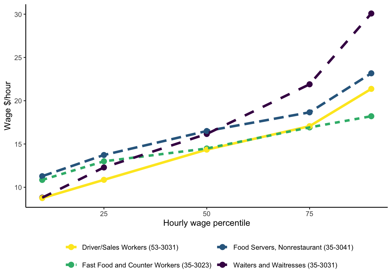
Source: Occupational Employment and Wage Statistics (US)

Another possible explanation for variation in observed wages could be that wages in some sectors are affected by market imperfections.

First, we could think about market power. When employer is operating as a monopsonist (sole buyer of labour), then wages in that sector of the economy may be dampened. For example, compare the distribution of wages between workers in fast-food restaurants, waiters and food servers. Fast-food sector is more likely to contain large fast-food chains, which may be operating as monopsonists. (However, note that this can be very difficult to show). We see that hourly wages of fast-food workers are typically lower and more compact.

Second, market imperfections may also arise due to asymmetric information. When employers don’t observe exact productivity types of their workers, they will need to pay wages based on some kind of average information. It means that these wages may be above marginal productivities for some workers, and below - for others. It is again difficult to find a direct evidence in the data that we could attribute to this phenomenon. As a proxy, we could look at the wages of workers in food sector to those of food delivery workers (yellow line in the above figure). It may be interesting because productivity of delivery workers may be easier to measure, especially nowadays with delivery apps and rating scales so ubiquitous. In particular, interesting comparison is between wages of delivery workers and fast-food counter workers. We see that lowest wages of delivery workers are below the lowest wages of fast-food counter workers, and highest wages are above. This could point to the possibility that wage scheme of fast-food counter workers suffer from imperfect information.

Of course, there are many things happening at the same time, and none of the graphs above isolate one specific channel. But they give us some ideas of what might be happening.

We will now study the impact of compensating differentials and market imperfections on wages. In the end, we will review some of empirical papers that attempt to estimate the importance of different channels.

Perfect competition

Jobs of equal difficulty

• Production function \(F(L): F_L(L) = y\)

• Workers supply \(h=1\) unit of labour and receive wage \(w\) if hired

• Linear worker utility \(U(R, e, \theta) = R - e\theta\)

  • \(R = w\) if employed; \(R=0\) otherwise
  • \(e\) difficulty of jobs, \(e=1\) is constant
  • \(\theta \geq 0\) heterogeneous disutility (\(G_\theta(\cdot)\) CDF)

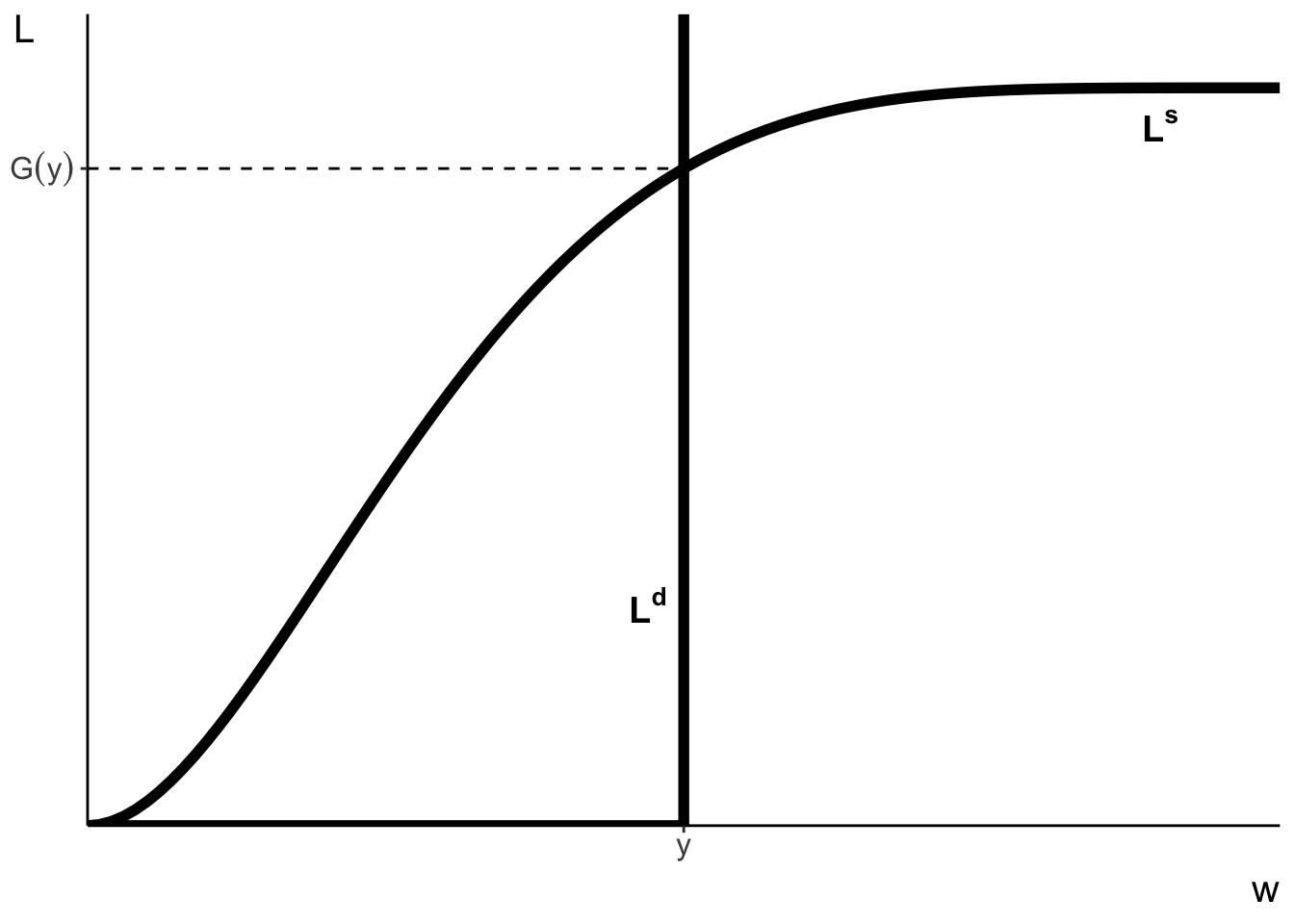
• Equilibrium

  \[ L^d = \begin{cases}+\infty & \text{if } w < y \\ [0, +\infty) & \text{if } w = y \\ 0 & \text{if } w > y\end{cases} \]

  \[ L^s = G(w) \]

We begin with a very simple model.

First, we specify single-input production function \(F(L)\) such that marginal productivity of each unit is constant \(F_L(L) = y\). We can write down profit function for the firm as \(F(L) - wL\), where price of output is normalized to 1. From this we know that optimal labour demand satisfies FOC \(y = F_L(L^\star) = w\). Note that we do have multiple solutions here: when \(w=y\), any amount of labour input will do. Therefore, the labour demand is given by the system shown above. If \(w < y\), the firm will want to hire all the labour there is. If \(w < y\), the firm has no interest in hiring anyone.

On the worker side, we also have a very simple case with utility that only depends on consumption and disutility of job \(U(C, e; \theta) = C - e\theta\). The budget constraint is super simple: \(C = w \cdot h\). The total time endowment is normalized to 1. Since there is no utility of leisure, the worker either supplies all time to work \(h=1\) or doesn’t work at all \(h=0\). Therefore, the utility of the worker can be written \(U(R, e; \theta) = w - e\theta\) if she works, and \(U(R, e; \theta) = 0\) otherwise. Therefore, she only decides to work if and only if \(w - e\theta \geq 0 \Rightarrow w \geq \theta\) (taking into account that we also normalised \(e = 1\) at the beginning). Remember that from the worker-point of view, \(w\) is given and each worker has her own \(\theta\). This is her innate preference for working that she is born with. Therefore, all workers with \(\theta < w\) find it optimal not to work, and the rest devote all their time to work.

\[ h^\star = \begin{cases} 1 & \text{if } w \geq \theta \\ 0 & \text{if } w < \theta\end{cases} \]

Since we know the distribution of \(\theta\), we can calculate how many workers in the economy will work.

\[ L^s = \Pr\left(\theta \leq w\right) = G(w) \]

Jobs of equal difficulty

We can also illustrate the equilibrium in graphical form. The figure above plots the optimal labour demand and labour supply curves as a function of wages.

As we said earlier, at any wage \(w < y\), the firm doesn’t want to employ anyone. Therefore, labour demand curve there is horizontal at zero. At \(w = y\), the firm is happy employing any amount of workers \(\Rightarrow\) it becomes a vertical line all the way up to infinity. Beyond this point, labour demand is infinite and cannot be drawn.

The labour supply curve is basically just the CDF curve at respective wages. We know that the CDF curve is increasing and bounded between 0 and 1.

It is easy to see that labour supply and demand curves cross only once at a point \(w = y\) and equilibrium employment in the economy is equal to \(G(y)\).

This is a super simple case where firms and workers don’t really make any decisions. However, it helps to setup the environment where we can now explore the role of job characteristics.

Jobs of varying difficulty

• Continuum of jobs with varying difficulty \(e > 0\)

• Productivity \(y = f(e)\) such that \(f^\prime(e) > 0, f^{\prime\prime}(e) < 0, f(0) = 0\)

• \(e\) also corresponds to effort worker puts in if employed

• Compensating wage differentials: \(w^\prime(e) > 0\)

  \[ L^d = \begin{cases}+\infty & \text{if } w(e) < f(e) \\ [0, +\infty) & \text{if } w(e) = f(e) \\ 0 & \text{if } w(e) > f(e)\end{cases} \]

  \[ L^s = \begin{cases} 1 & \text{if } f^\prime(e) = \theta \cap f(e) - e\theta \geq 0 \\ 0 & \text{otherwise} \end{cases} \]

Now, we can consider a case where jobs do vary in the type and difficulty of tasks they involve. We assume that all relevant characteristics of the job can be summarised in a uni-dimensional variable \(e > 0\).

Important addition is that now the characteristic \(e\) is relevant for production function. In particular, marginal productivity of labour is no longer constant, but increasing function of \(e\): \(F_L(L) = y = f(e)\). Therefore, every job with different \(e\) will have their own wage \(w(e)\) in the equilibrium. The labour demand of a firm with job of difficulty \(e\) will still look very similar to the demand curve we’ve seen on the previous slide. If \(w(e) < f(e)\), then firm wants to employ as many people as possible. If \(w(e) = f(e)\), then firm is indifferent between any amount of labour as FOC is satisfied at any \(L\). If \(w(e) > f(e)\), then firm has no interest in employing anyone.

The worker chooses which job to supply her labour to. Once she has chosen a job with characteristic \(e\), she has to do all the required tasks. So, in a way, the variable \(e\) also captures the effort she has to exert to do this job. Her utility function has the same form as before. Therefore, if she works at job \(e\) she gets utility \(w(e) - e\theta\) and if she doesn’t work she still gets utility of zero. Therefore, she would only work if \(f(e) - e\theta \equiv w(e) - e\theta \geq 0\). This time, apart from deciding to work or not, she can also choose the job at which she wants to work. The optimal job \(e^\star\) should satisfy the FOC

\[ f^\prime(e^\star) = \theta \]

To make sense of this condition imagine what happens if she works at jobs with slightly lower \(e\) or slightly higher \(e\). With slightly lower \(e\), she is in a situation where the job is not too difficult for her. Her disutility parameter \(\theta\) allows her to tolerate even more difficult jobs, and by doing so, she could also earn higher wages. Therefore, it is not optimal for her to work at less difficult jobs. If she, however, works at a job with a higher \(e > e^\star\), then it is too difficult for her. Even though she’s getting higher wages, her disutility from that job outweighs higher consumption utility.

We can also describe the relationship between \(e^\star\) and \(\theta\). Using implicit function differentiation of the FOC above, we can show that

\[ \frac{\text{d}e^\star}{\text{d}\theta} = \frac{1}{f^{\prime\prime}(e^\star)} < 0 \]

Meaning that higher is the disutility parameter of the worker \(\theta\), the less difficult her optimal job \(e^\star\) is. It makes sense: if the worker really hates putting in a lot of effort, she doesn’t want to choose very difficult jobs.

Notice also that wages are increasing in difficulty \(w^\prime(e) > 0\). This is because in the equilibrium, \(w(e)=f(e)\) and we have assumed that marginal productivity is increasing in \(e\). This is called compensating differentials. Jobs with “worse” characteristics have to compensate their workers with higher wages.

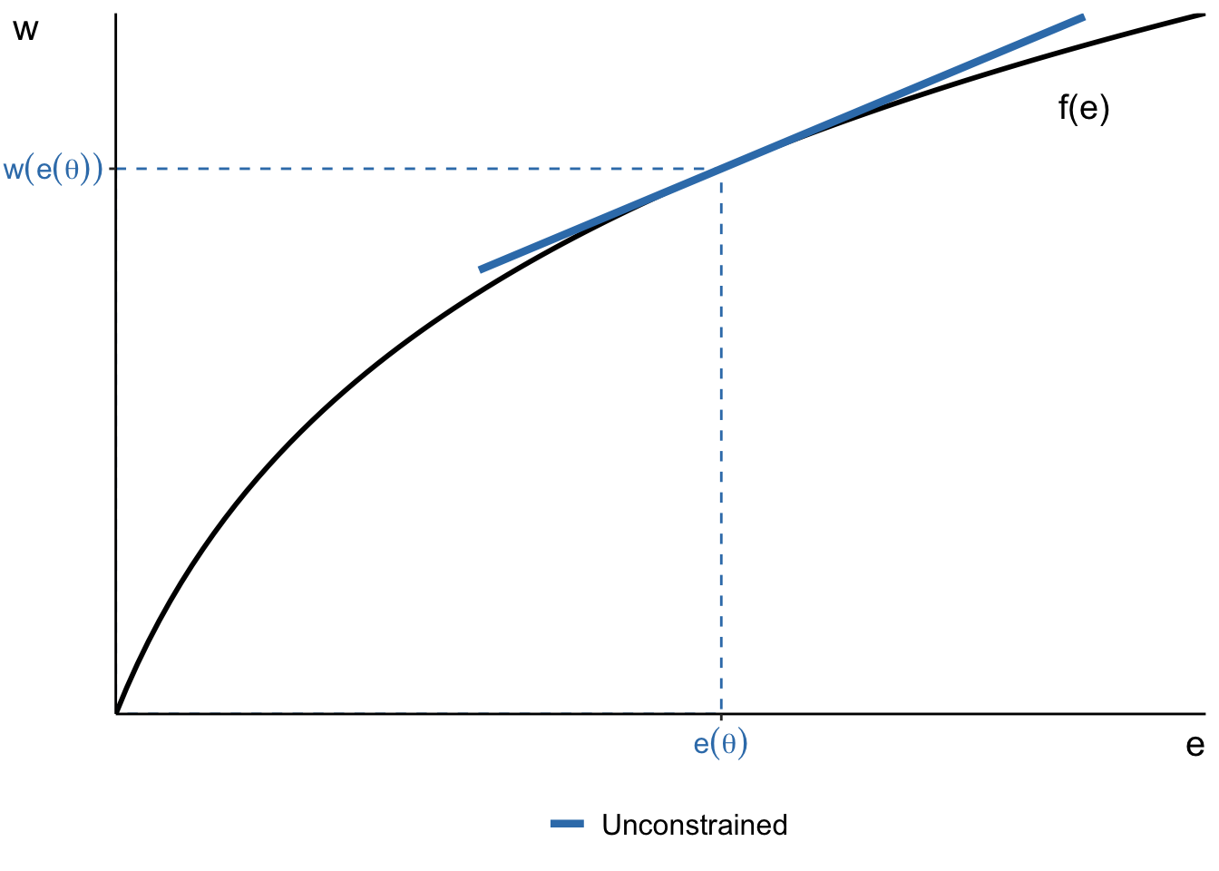
Jobs of varying difficulty

We can illustrate the optimality conditions graphically in the \(w\)-\(e\) space.

Recall that we assumed a simple linear utility function. It implies that indifference curve between \(w\) and \(e\) is a straight line with slope \(\theta\).

And we can also plot the production function in the same space. It is increasing and concave.

Now, consider two workers: one with low \(\theta_L\) (blue) and one with high \(\theta_H\) (red). The low type will have shallower indifference curve and the high type - steeper. Because the marginal productivity curve is concave, the tangency point with the low-type indifference curve occurs at higher \(e(\theta_L)\) than with the high-type indifference curve (at \(e(\theta_L)\)).

This is exactly what the optimality condition equations are describing. Workers with \(\theta_L\) choose jobs of higher difficulty \(e(\theta_L)\) and earn higher wages \(w(\theta_L)\). Workers with higher disutility parameter \(\theta_H\) choose easier jobs \(e(\theta_H) < e(\theta_L)\), but earn lower wages \(w(\theta_H) < w(\theta_L)\).

Wage dispersion: compensating differentials

This is one of the potential explanations why observed wages in the economy may vary from worker to worker. Even if you fix individual worker productivities and assume they are all capable of doing each job, workers may still have varying preferences for different aspects of jobs. Knowing this employer may offer higher wages for less attractive jobs.

Workplace safety regulation

At baseline worker of type \(\theta\) chooses optimal effort \(e(\theta)\) and earns \(w(e(\theta))\)

We can also analyse the predictions of this model when the policy makers put in place workplace safety regulations.

First, let’s re-draw the optimal choice of job and equilibrium wage of a worker with \(\theta\) without any safety regulations. This worker will choose a job \(e(\theta)\) and be paid \(w\left(e\left(\theta\right)\right)\).

How can we illustrate safety regulation such that no work can be of difficulty \(\bar{e} < e(\theta)\)?

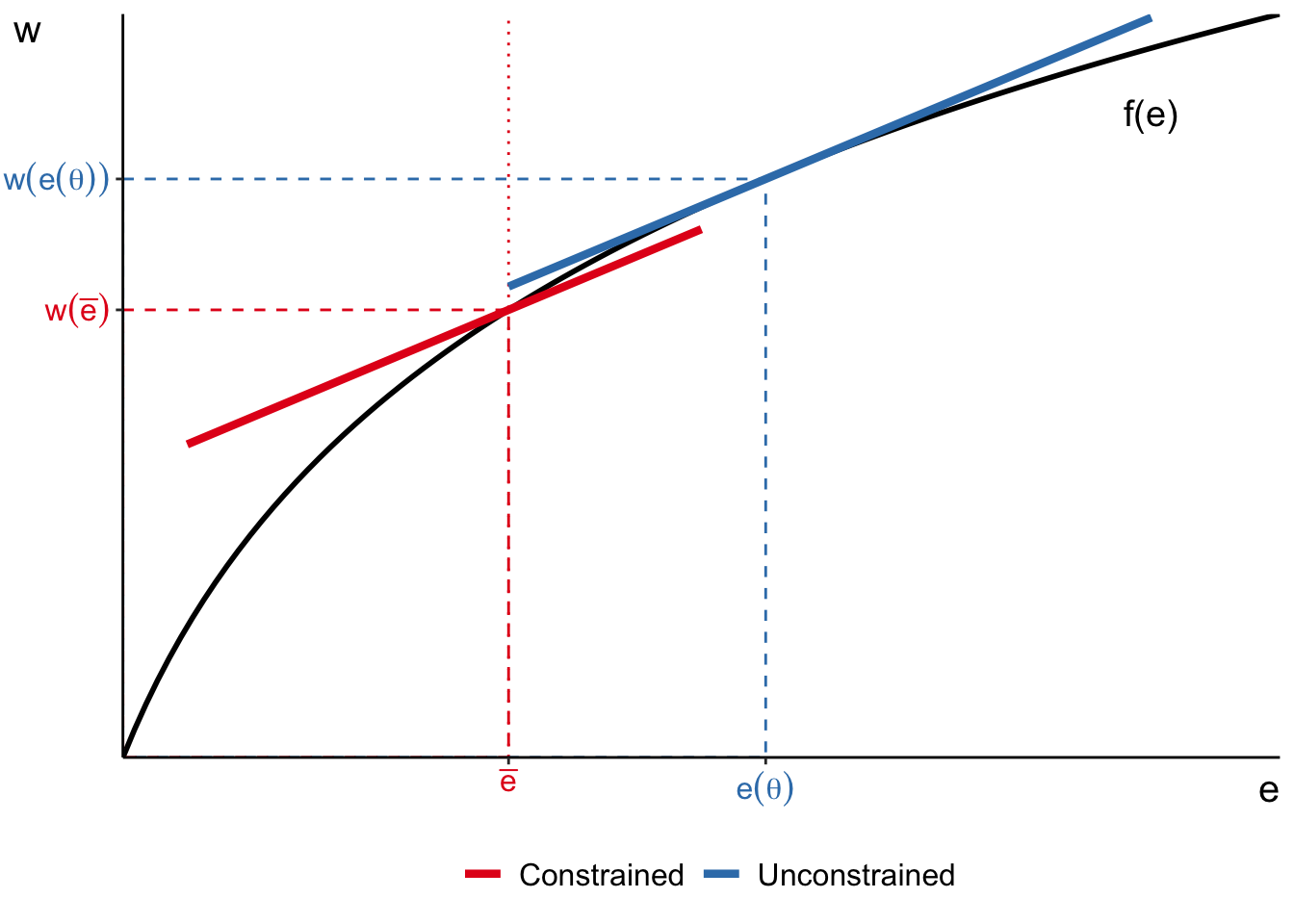
Workplace safety regulation

Limit on job difficulty \(\bar{e}\) forces worker type \(\theta\) on a lower indifference curve

Now, the jobs cannot be more difficult than \(\bar{e}\). For the worker we consider, \(\bar{e} < e(\theta)\). So, she is forced to work at a job that is too easy for her, and she gets paid \(w(\bar{e})\) instead of \(w(e(\theta))\). We can see that it is suboptimal because her indifference curve has to shift down so that it crosses the marginal product line at the point \(\bar{e}\). There is no point in shifting the indifference curve even lower because then she gets even less utility.

Notice that under perfect competition, having workplace safety regulation makes workers worse off! Because under perfect competition, workers have full information about perils of job and own skills, and choose accordingly. For example, \(w(e(\theta))\) should also be compensating for increased healthcare costs if job is very dangerous.

However, the equilibrium with \(e(\theta)\) and \(w(e(\theta))\) may not be attainable with imperfect competition! In this case, workplace safety regulations can improve the overall wellbeing of workers.

Perfect competition: summary

• Even under perfect competition, wages and labour supply decisions of workers depend on
  • abilities of workers: more productive workers earn higher wages
  • characteristics of jobs: more difficult jobs offer higher wages
• Efficient allocation of resources
  • part of the population may choose not to work because jobs are not attractive enough

Imperfect competition

Barriers to entry: monopsonistic employer

Start from baseline model

• Continuum of workers \(\theta\) with utility \(U(R, e, \theta) = R - e\theta, ~ e = 1\)
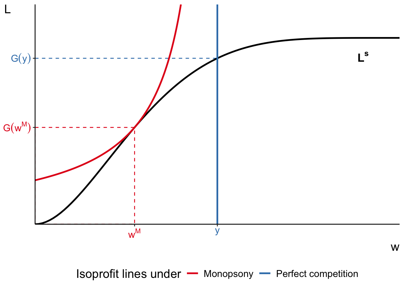
• Monopsonistic employer \(\max_w \pi(w) \equiv \max_w L^s(w) (y - w)\)

Equilibrium wage \(w^M = y\frac{\eta^L_w(w^M)}{1 + \eta^L_w(w^M)}\) where \(\eta^L_w(w^M) = \frac{w^M}{L^s(w^M)}\frac{\text{d}L^s(w^M)}{\text{d}w}\)

Equilibrium employment \(L^s(w^M) = G(w^M)\)

Labour markets may not operate under perfect competition. In this case, wages do not only reflect marginal productivities and individual preferences.

One example of imperfect competition is when the assumption of free entry fails. For example, workers may not be able to choose jobs and firms because there is only one employer in her labour market. Barriers to entry may arise due to geographic isolation or licencing costs of heavily-regulated jobs.

We will continue with a simple linear utility function of the worker. For simplicity, we again assume that \(e\) is constant and normalize it to 1. So, we know that the agent works if her \(\theta \leq w\) and doesn’t work otherwise.

On the firm side, we again assume constant marginal product of labour \(y\). So, the firm’s profit is \(Ly - wL\). Because firm is a monopsonist, its labour demand will determine the equilibrium employment in the economy. We already take that into account by using labour supply \(L^s\) directly in its profit equation. Then, the firm needs to set the wage that would maximise its profit.

Monopsonistic wage derivation (FOC)

\[\begin{align} 0 &= \frac{\text{d}L^s(w^M)}{\text{d} w}\left(y - w^M\right) - L^s(w^M) \\ 1 &= \frac{y}{w^M}\frac{w^M}{L^s(w^M)}\frac{\text{d}L^s(w^M)}{\text{d}w} - \frac{w^M}{L^s(w^M)}\frac{\text{d}L^s(w^M)}{\text{d}w}\\ 1 &= \frac{y}{w^M} \eta^L_w(w^M) - \eta^L_w(w^M)\\ w^M &= y\frac{\eta^L_w(w^M)}{1 + \eta^L_w(w^M)} \end{align}\]

Since \(\frac{\text{d}L^s(w^M)}{\text{d}w} = \frac{\text{d}G(w^M)}{\text{d}w} > 0\) (thanks to \(G(\cdot)\) being a CDF), the labour supply elasticity to wage is also positive \(\eta^L_w(w^M) > 0\).

This means that \(\frac{\eta^L_w(w^M)}{1 + \eta^L_w(w^M)} < 1 \Rightarrow w^M < y = w^{PC}\). Wages paid to workers by a monopsonistic employer are lower than wages paid in perfectly competitive labour market.

We can use this expression to define monopsony power as the ratio between marginal productivity (i.e., wage under perfect competition) and monpsony wage, \(\frac{y}{w^M}\). It is also clear that the monopsony power clearly depends on the elasticity of labour supply with respect to wages. If it is highly elastic \(\eta_w^L = 1\), then monopsonist cannot offer wages that are too low and has to take into account the falling employment. If labour supply is highly inelastic \(\eta_w^L = 0\), then monopsonist can set wages “arbitrarily” low.

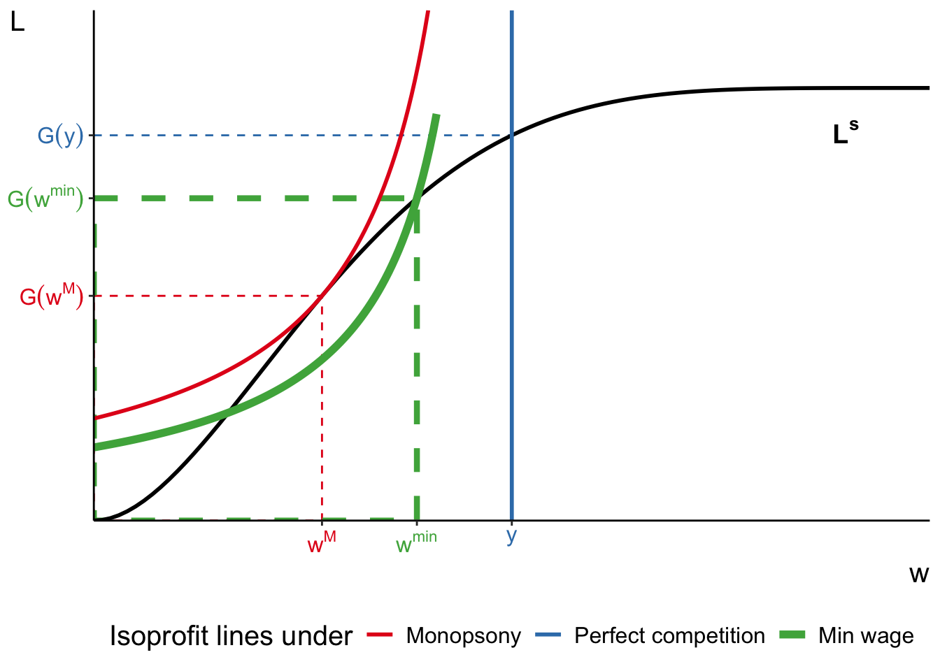
Barriers to entry: monopsonistic employer

If we represent this labour market in graph, then the monopsonistic equilibrium is found at the point of tangency between the labour supply curve and isoprofit line. We can see clearly that \(w^M < w_{PC}=y\) and equilibrium employment is \(G(w^M) < G(y)\).

Monopsonistic employer and minimum wage

What happens if government mandates min wage \(w^M < w^\text{min} < y\)?

Monopsonistic employer and minimum wage

Equilibrium employment and wages both rise!

Recall from lecture 3, we discussed briefly how minimum wages can have positive effect on employment in monopsonistic labour markets. We can use our current setting to understand why.

Assume that the government mandates \(y > w^\min > w^M\). In this case, the isoprofit line of the firm has to shift down until it cross the labour supply curve at \(w^\min\). Because \(w^\min > w^M\) and labour supply is increasing function of \(w\), we can also see that equilibrium employment rises \(G(w^\min) > G(w^M)\).

Can you describe how the equilibrium changes in this market when \(w^\min > y\)?

Imperfect information and adverse selection

• Workers are now described by their ability \(h > 0\) with CDF \(G(\cdot)\)
  • produce \(h\) units of good
  • enjoy leisure utility \(d(h)\) such that \(d^\prime(h) > 0\) and \(d(h) < h\)
• Workers enjoy utility \(U(R, d) = \begin{cases} w(h) & \text{if hired}\\ d(h) & \text{otherwise}\end{cases}\)
• Firms now offer identical jobs \(e = 1\) and \(\max_L \mathbb{E}\left[(h - w(h))L\right]\)
• Firms do not observe true \(h\) of workers (only see the distribution \(G(\cdot)\))

Another form of market failure that can affect wage setting arises due to imperfect information.

We have seen in the previous lecture the case where workers have imperfect information about jobs. There workers could end up with different wages even though their marginal productivities and preferences are identical. We also briefly discussed the implications of an extension where firms are added to the search model. In particular, one of the implications was that firms were willing to offer higher wages when competition for workers is high. This could also be reflected in the wages of a worker with longer working history being much higher than wages of a new entrant, even if their marginal productivities are exactly the same.

This time we will consider what happens to the firm behaviour when they don’t have enough information about workers.

In this model, workers have different abilities \(h\). You can think that worker of type \(h\) has marginal productivity \(h\). Firms do not know the true type of worker, but they do know the distribution of worker types in the economy. We also assume that a productive worker (high \(h\)) is also more productive at home. Therefore, her leisure utility \(d(h)\) is also an increasing function of \(h\). To ensure that workers have incentives to be employed, we also assume \(d(h) < h\).

Can you describe the equilibrium in this model under perfect perfect competition and full information?

Firms now offer identical jobs (\(e=1\)). Because they don’t observe true marginal productivities of their labour force, firm’s have to maximise expected profit. There exist equilibria in this model where the wage schedule \(w(h)\) depends on type \(h\). But in the following slides we will consider pooling equilibrium, where firms do not attempt to discern worker types.

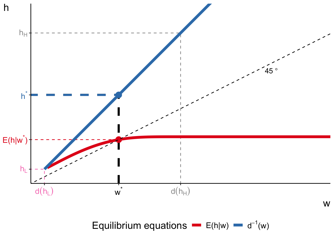
Imperfect information and adverse selection

Equilibrium is described by a pair \((w^\star, h^\star)\) such that

• all workers with \(h < h^\star = d^{-1}(w^\star)\) decide to work
• firms hire all workers ready to work at \(w^\star = \mathbb{E}\left(h | w^\star\right)\)

We can graphically illustrate the equilibrium by plotting \(d^{-1}(w)\) and \(\mathbb{E}\left(h | w\right)\) on the next slide

The FOC of the firm problem is \(w = \mathbb{E}(h)\). Meaning that equilibrium wage is equal to average marginal productivity. However, we have to account for the fact that not all workers might be willing to supply their labour in this equilibrium. Therefore, the correct way of writing down the FOC of the firm problem is

\[ w^\star = \mathbb{E}\left(h | w^\star\right) \]

That is, equilibrium wage is equal to expected marginal productivity of workers conditional on them being ready to work at \(w^\star\).

A worker of type \(h\) decides to work at \(w^\star\) iff \(d(h) < w^\star\). Since \(d(\cdot)\) is increasing function, we can also write the decision rule as

\[ h < d^{-1}\left(w^\star\right) \equiv h^\star \]

Therefore, the equilibrium labour supply in the economy is \(G\left(d^{-1}\left(w^\star\right)\right)\).

It also means that average production at firm is

\[ \mathbb{E}\left(h | w\right) = \frac{\int_0^{d^{-1}(w)} zdG(z)}{G\left(d^{-1}\left(w\right)\right)} \]

Imperfect information and adverse selection

Here, we represent the equilibrium in \(h\)-\(w\) space.

First, we can draw for every possible \(w\), the expected marginal productivity of workers ready to work at that wage. This is given by the red line in the plot above. Recall that optimal wage is found from \(w^\star = \mathbb{E}\left(h | w^\star\right)\). That point is found at the intersection of \(E\left(h|w\right)\) curve with a 45° line.

Second, we can also draw \(d^{-1}\left(w\right)\) at every possible \(w\). This is given by the blue line in the plot. Once we know the optimal \(w^\star\), we can find \(h^\star\) from this curve.

You can now clearly see how imperfect information changes equilibrium. All workers of type \(h < \mathbb{E}\left(h | w^\star\right)\) obviously want to work because their wage is now much higher than what they would have earned under full information. All workers of type \(\mathbb{E}\left(h | w^\star\right) \leq h \leq h^\star\) still want to work because their utility of leisure is not sufficiently high, but they get underpaid.

Another important observation is that pooling equilibrium will exclude the most productive workers from the labour market. All workers of type \(h > h^\star\) are not interested in working because the wage schedule offered does not compensate them enough. You can see that workers with very high \(h\) get underpaid a lot more severely than workers with lower \(h\).

Finally, let’s assume that worker types are bound between \([h_L, h_H]\). If firms wanted to save cost and offer wages \(w=d(h_L)\), then no worker will be interested in working. Conversely, if firms were to offer wages \(w=d(h_H)\), then all workers would be interested in supplying their labour. However, firm would find itself making losses from production.

There exists another, separating equilibrium, where firms can use costly unproductive signals to discern worker types. In that case, the firm is able to offer wage schedule equivalent to that under full information (pay each worker their marginal productivity). In this case, workers must bear the cost of the signal.

Imperfect competition: summary

Wages no longer reflect productivity differences alone

• monopsonistic employer: equilibrium wages and employment \(\downarrow\)
  • innovation and mobility costs (Cahuc 2004, ch 5.2)
  • trade unions (Cahuc 2004, ch 7)
• Workers and firms may have incomplete information about each other
• In the example, where firms do not know true worker productivities
  • \(w^\star\) may be too high for some workers and too low for others
  • adverse selection: most productive workers stay unemployed
• Last lecture, workers have imperfect information about jobs
  • with on-the-job search and endogenous wages, \(w > y\) for senior workers

Empirical evidence

Estimates of compensating differentials

Regression of wage \(w\) on job difficulty \(e\)

\[ \ln w_i = \mathbf{x}_i \boldsymbol{\beta} + \mathbf{e}_{J(i)} \boldsymbol{\alpha} + \varepsilon \]

• \(\mathbf{x}_i\) - observed worker characteristics
• \(\mathbf{e}_{J(i)}\) - observed job characteristics of worker \(i\)

Early estimates biased by

• unobserved heterogeneity in productivity
• unobserved heterogeneity in preferences

For example,

• \(\mathbf{x}_i\) may contain gender, age, educational qualifications/years of education, work experience, ethnicity, place of residence, family status, trade union membership, etc.
• \(\mathbf{e}_{J(i)}\) may contain duration of contract, flexibility of hours worked, task content, risk of injury, noise levels, physical strength required by the job, risk of losing the job, cost of health insurance, cost of retirement savings, etc.

Ideally, \(\boldsymbol{\alpha}\) captures the compensating differentials effect. However, unobserved individual heterogeneities may put downward bias to the estimates of compensating differentials, or even change sign of \(\boldsymbol{\alpha}\).

• Workers may rank job characteristics differently: some workers might like jobs with high physical strength requirements, and others - not.
• This means that there may not be universally agreed ranking in \(e_{J(i)} \Rightarrow\) not obvious what wages are compensating
• Workers may differ in their productivities, which allows them to choose jobs of lower difficulty while still enjoying higher income (see illustration on next slide).

Estimates of compensating differentials

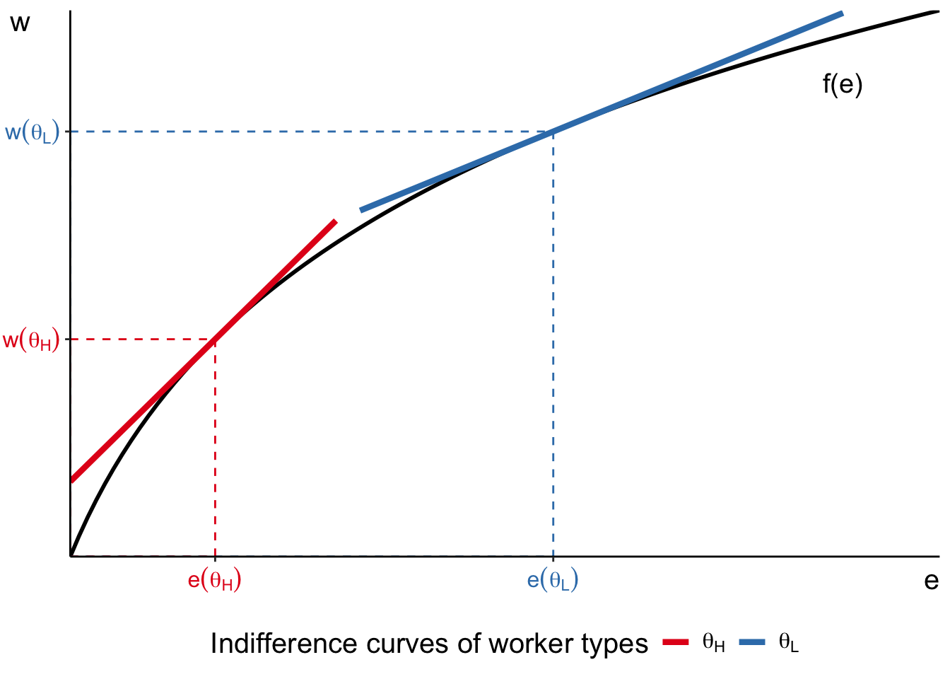
Unobserved heterogeneity in productivity

Consider again model with varying \(e\) and two workers with \(f_H(e), f_L(e)\)

Let’s consider again the model with jobs of varying difficulty. Imagine that we have two workers with identical disutility parameter \(\theta\). Remember that \(\theta\) is also slope of their indifference curves.

The optimal job choice of workers is at the point where their marginal productivities are equal to their disutility parameter \(\theta\). So, graphically, that happens at the tangency between indifference and marginal productivity curves.

Workers only differ in their productivities. Let’s say that red worker is less productive at every job and blue worker is more productive at every job. It means that marginal productivity curve of the blue worker is higher. Therefore, the optimal job choice and wages of red and blue workers will be different and depend on the curvature of utility and productivity functions.

The case illustrated above suggests that more productive guy choose a less difficult job and earns higher wages. So, even if both of these workers have same \(\theta\) (i.e., compensating differentials should work the same way for them), if we do not observe their productivities, the simple regression will suggest negative relationship between \(e\) and \(w\).

• The optimal effort \(e_H < e_L\). Think about income effect.
  • Worker \(H\) earns a lot more for any given effort \(e\)
  • Since \(e\) is costly and generally undesirable, worker \(H\) can afford to choose job with lower \(e\) without losing too much in income.
• Note that compensating differentials still holds in this illustration.
  • if you fix the productivity level and allow workers to differ by \(\theta\), then workers with lower \(\theta\) will choose higher \(e\) and earn higher \(w\)
• Hence, failing to account for individual heterogeneity in productivity biases the slope of \(w\) with respect to \(e\) downwards.

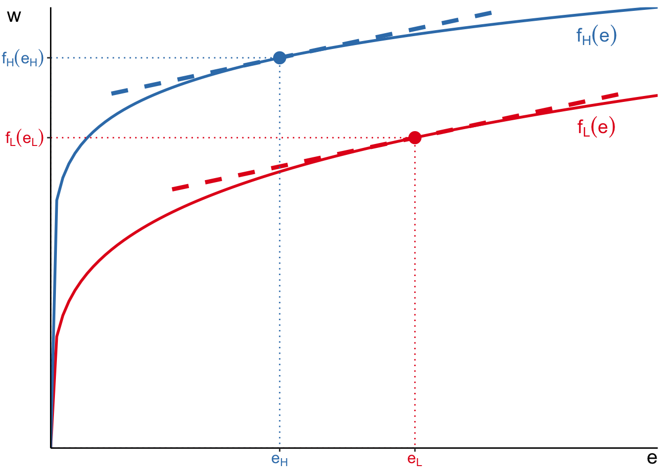
Estimates of compensating differentials

Hwang, Reed, and Hubbard (1992)

	Thaler and Rosen (1976)	Hwang et al. (1992)
Age	3.890	4.500
	(0.800)
Age \(^2\)	-0.048	-0.096
	(0.009)
Education	3.400	4.870
	(0.550)
Risk	0.035	0.302
	(0.021)
R2	0.41	0.31
Price of life saved (in years of wage)	26.54	227.67
Mean weekly wage	132.65	132.65

• Early estimates from cross-sectional data taken from Thaler and Rosen (1976)
• According to these estimates, reducing the risk of death is worth 26.54 years of work at average wage.
• Hwang, Reed, and Hubbard (1992) illustrate how these estimates suffer from unobserved heterogeneity (both in preferences and productivities)
• Then Hwang, Reed, and Hubbard (1992) make assumptions about model parameters that capture these heterogeneities based on existing evidence. That is, these parameters should closely approximate real labour markets.
• Under these parameter assumptions, the price of life saved rises to 227.67 years of work at average wage!

Estimates of compensating differentials

Bonhomme and Jolivet (2009)

Job search frictions: even small costs enough MWP \(\neq\) wage differentials

	Finland
	MWP	Wage differentials
Type of work	0.016	0.107
	(0.180)	(0.040)
Working conditions	0.070	0.004
	(0.080)	(0.030)
Working times	-0.016	0.048
	(0.070)	(0.040)
Distance to work	0.162	-0.031
	(0.060)	(0.040)
Job security	0.537	0.068
	(0.220)	(0.040)

• Searching and changing jobs may be too costly, so workers may not switch to a better job if the benefit is too small
• There may be incomplete information about jobs, so workers do not know fully which job is optimal
• In addition, Bonhomme and Jolivet (2009) allow for unobserved heterogeneity in productivities and preferences
• The authors show that
  • in cross-sectional wage regressions, even with very small job search costs estimated wage differentials have no resemblance to underlying individual preferences for amenities (MWP)
  • dynamic regressions based on job changes can reflect individual preferences for amenities, but only if all job changes were voluntary
  • even a small share of involuntary changes “makes preferences almost invisible” in estimates of wage differentials

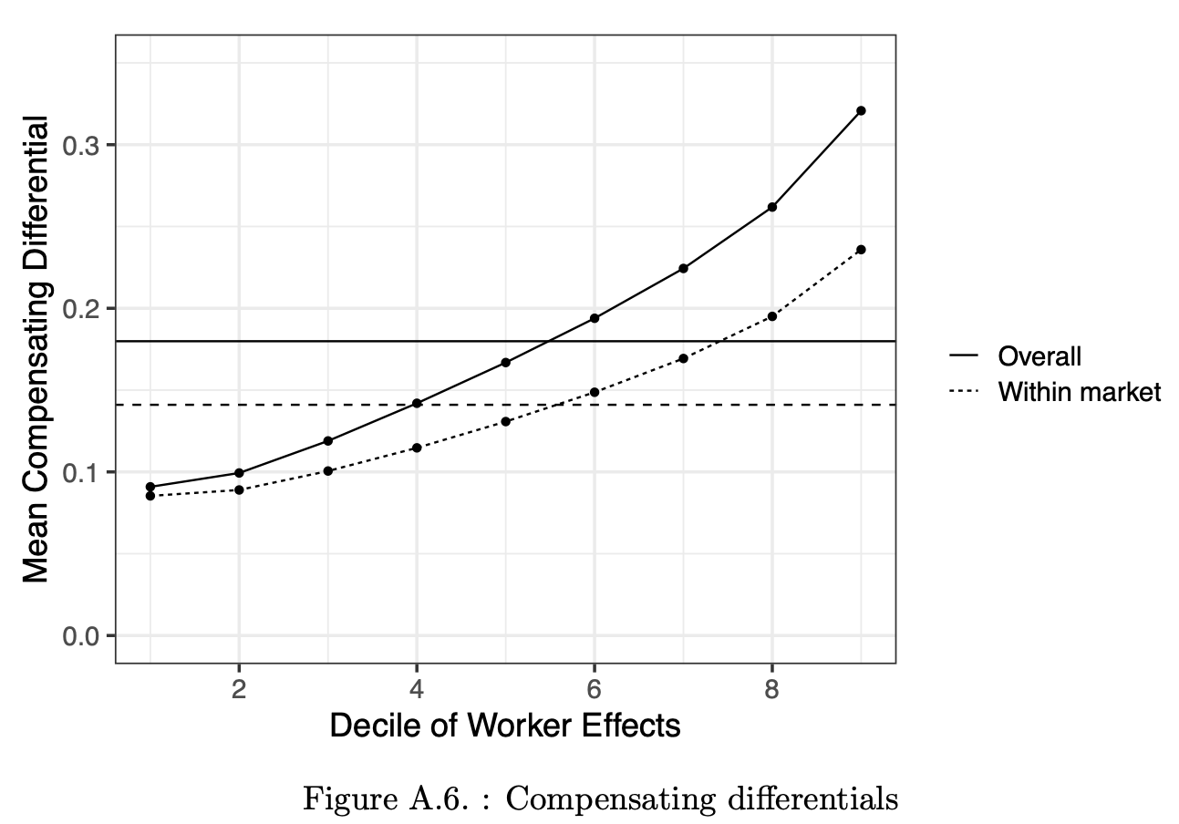
Estimates of compensating differentials

Lamadon, Mogstad, and Setzler (2022)

• Lamadon, Mogstad, and Setzler (2022) aim to quantify the importance of imperfect competition in explaining the labour market patterns in the US.
• They do so by quantifying the amount of rents firms and workers extract from ongoing employment relationships
• To be able to estimate the rents, the model needs to allow heterogeneity in preferences for non-wage amenities
• As a result, also can estimate the magnitude of compensating differentials that describe the data
• The authors report sizeable differentials
  • on average, firms have to pay 10-30% higher wages to compensate for less attractive jobs
  • interesting that this number is increasing in worker productivities!

Determinants of wage inequality

Taber and Vejlin (2020)

Estimate importance of four channels of wage heterogeneity:

• Roy model: comparative advantage in skill for job
• Job search model: search and mobility costs
• Compensating differentials model: preferences for non-wage attributes
• Human capital model: boost productivity while working

• Roy model: choose jobs according to absolute and comparative advantage in individual skills
• Job search model:
  • workers may not have met the firm/job that is most optimal to them \(\Rightarrow\) have to settle for sub-optimal choices
  • workers may not have enough bargaining power at the optimal firm because they don’t have good enough alternative job offers
• Compensating differentials: accept lower wages for a job that worker enjoys more
• Human capital: accumulate more human capital (that raises productivity) while working

Separating between the different determinants of wage inequality is important from the policy perspective too.

• If most of inequality comes from compensating differentials (i.e., individual preferences), we may not want to correct for it
• If wage inequality is mostly explained by differences in pre-market skills (Roy model), then policies targeted at childhood development, schools and education system are appropriate.
• If wage inequality is driven by job search frictions, then optimal policies should try to correct for these issues (for example, online job portals, standardised CV screenings, blind auditions etc)
• If wage inequality is mostly due to human capital accumulation while working, then we may want to implement policies that make on-the-job training more accessible, better structured, more targeted, etc.

Determinants of wage inequality

Taber and Vejlin (2020)

A	Variance
Total	0.104
No learning by doing	0.096
No monopsony	0.093
No premarket skill variation across jobs	0.05
No premarket skill variation at all	0.008
No search frictions	0.007

B	Variance
Total	0.104
No learning by doing	0.096
No monopsony	0.093
No search frictions	0.086
No premarket skill variation across jobs	0.049
No premarket skill variation at all	0.007

C	Variance
Total	0.104
No learning by doing	0.096
No monopsony	0.093
No nonpecuniary aspects of jobs	0.087
No premarket skill variation across jobs	0.048
No premarket skill variation at all	0.006

D	Variance
Total	0.104
No learning by doing	0.096
No monopsony	0.093
No nonpecuniary aspects of jobs	0.087
No search frictions	0.061
No premarket skill variation across jobs	0.047

• The relative importance of each factor is measured by the reduction in variance of log wages after removing that factor.
• Therefore, the importance estimates depend on the order in which different factors are removed \(\Rightarrow\) four scenarios.
• In all four cases, human capital accumulation on the job and monopsony power are removed first since these are expected to be small in magnitude based on existing studies.
• In all four scenarios, premarket variation in skills is by far the most important factor, explaining between 50-80% of variation in wages.
• Search frictions explain between 1-26% of wage variations depending on the order of elimination.
• In these scenarios, compensating differentials do not explain much of wage inequality.
• However, in Table VII Taber and Vejlin (2020) show that compensating differentials are extremely important for explaining utility variations and job choices!

Determinants of wage inequality

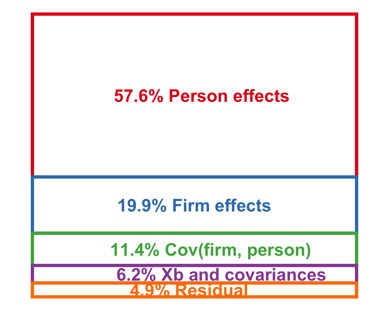
Firm-specific wage premiums

Firms may pay different wages to otherwise identical workers

\[ Y_{it} = \beta_0 + \boldsymbol{\beta}_1 \mathbf{X}_i + \theta_i + \psi_{J(i)} + \varepsilon_{it} \]

• Card, Cardoso, and Kline (2016): ~20% of wage inequality due to firm premium
• Song et al. (2019): completely explained by sorting and segregation of workers
• Bonhomme et al. (2023): bias-corrected contribution 5-13%

• Another direction of research in wage inequality explores the firm premiums.

• The observation in the data is that observationally equivalent workers (i.e., with similar observed skills) earn different wages if they work in different firms.

• Abowd, Kramarz, and Margolis (1999) provide an easy regression-based decomposition of wages into observable worker characteristics, unobservable worker premiums, unobservable firm premiums and residuals. This decomposition is generally known as AKM decomposition.

• Using this decomposition framework, Card, Cardoso, and Kline (2016) show that nearly 20% of total wage variation is attributable to variation in firm premiums.

• That is, there are firms that generally pay higher wages to all its workers and firms that generally pay lower wages.

• It is ongoing area of research with mixed results.

• For example, Song et al. (2019) argue that all of the observed firm effects are completely explained by worker sorting and segregation. That is,

  • more productive workers tend to work in higher-paying firms (worker sorting), and
  • more productive workers tend to work with other more productive workers (worker segregation)

  Hence, if these two channels are shut down (so worker composition is comparable between firms), then firm premiums would vanish.

• Bonhomme et al. (2023) illustrate that the AKM decomposition is biased by limited mobility in the data.

  • The identifying variation in the decomposition comes from workers that change workplaces.
  • However, the set of workers that change employers may be different from the general set of all workers.
  • Therefore, the decomposition may overestimate the importance of firm effect.

• They report bias-corrected estimates of contribution of firm premiums to overall wage inequality between 5-13%.

Summary

• Wage dispersion can be related to
  • individual heterogeneity in productivity/job tastes
  • heterogeneity in job conditions
  • monopsonistic employers forcing wage \(\downarrow\) for some workers
  • seniority premium with incomplete information and labour market costs
• Incomplete information can also drive most productive workers out
• Differentiating between different channels in data can be challenging

Next lecture: Human Capital on 10 Sep

References

Abowd, John M., Francis Kramarz, and David N. Margolis. 1999. “High Wage Workers and High Wage Firms.” Econometrica 67 (2): 251–333. https://www.jstor.org/stable/2999586.

Bonhomme, Stéphane, Kerstin Holzheu, Thibaut Lamadon, Elena Manresa, Magne Mogstad, and Bradley Setzler. 2023. “How Much Should We Trust Estimates of Firm Effects and Worker Sorting?” Journal of Labor Economics 41 (2): 291–322. https://doi.org/10.1086/720009.

Bonhomme, Stéphane, and Grégory Jolivet. 2009. “The Pervasive Absence of Compensating Differentials.” Journal of Applied Econometrics 24 (5): 763–95. https://doi.org/10.1002/jae.1074.

Cahuc, Pierre. 2004. Labor Economics. Cambridge (Mass.): MIT Press.

Card, David, Ana Rute Cardoso, and Patrick Kline. 2016. “Bargaining, Sorting, and the Gender Wage Gap: Quantifying the Impact of Firms on the Relative Pay of Women.” The Quarterly Journal of Economics 131 (2): 633–86. https://www.jstor.org/stable/26372650.

Hwang, Hae-shin, W. Robert Reed, and Carlton Hubbard. 1992. “Compensating Wage Differentials and Unobserved Productivity.” Journal of Political Economy 100 (4): 835–58. https://www.jstor.org/stable/2138690.

Lamadon, Thibaut, Magne Mogstad, and Bradley Setzler. 2022. “Imperfect Competition, Compensating Differentials, and Rent Sharing in the US Labor Market.” American Economic Review 112 (1): 169–212. https://doi.org/10.1257/aer.20190790.

Song, Jae, David J Price, Fatih Guvenen, Nicholas Bloom, and Till von Wachter. 2019. “Firming Up Inequality*.” The Quarterly Journal of Economics 134 (1): 1–50. https://doi.org/10.1093/qje/qjy025.

Taber, Christopher, and Rune Vejlin. 2020. “Estimation of a Roy/Search/Compensating Differential Model of the Labor Market.” Econometrica 88 (3): 1031–69. https://doi.org/10.3982/ECTA14441.

Thaler, Richard, and Sherwin Rosen. 1976. “The Value of Saving a Life: Evidence from the Labor Market.” In Household Production and Consumption, by Nestor E. Terleckyj, 265–302. NBER. https://www.nber.org/books-and-chapters/household-production-and-consumption/value-saving-life-evidence-labor-market.