3. Labour Demand

KAT.TAL.322 Advanced Course in Labour Economics

Nurfatima Jandarova

September 1, 2025

Labour demand

Firm decisions about how much labour to hire

Static model

Single factor input

Production function $Y = F(L)$ where $F^\prime > 0$ and $F^{\prime\prime} < 0$

\[ \max_{L} PF(L) - WL \]

FOC: $F^\prime(L) = \frac{W}{P}$

Downward-sloping labour demand

\[ \frac{\partial L}{\partial W} = \frac{1}{PF^{\prime\prime}(L)} < 0 \]

We begin from the static theory of labour demand.

A firm produces good $Y$ using $L$ as input and technology $F(L)$. The production function is increasing in $L$, but every additional unit of labour adds less and less to the production. Think of a bakery that initially had only one baker. Let’s say she could make 100 buns a day. If another person is hired, she could maybe help prepare twice as much dough. However, the bakery still has one oven. Therefore, maybe the total production of buns rises by only 50 more buns a day. And so on.

Note that in this version of the model there is no capital. This is equivalent to introducing capital in the model that is fixed and cannot be adjusted. In the example, the bakery needs to have physical facilities such as building and oven. Typically, physical capital is not easy to adjust on a day-to-day basis. For this reason, you can also use the model without capital to describe short-run behaviour of firms. On the next slide we will see the model where capital can be adjusted together with labour input.

The firm then sells its product $Y$ at price $P$ and pays wages $W$ to its personnel. As usual, we assume that firms’ objective is profit maximisation. We also assume here that firms are price-takers with respect to both $P$ and $W$. We can easily right down firm’s maximisation problem and first-order condition.

The FOC indirectly characterizes the labour demand function (if you assume a specific functional form of $F(\cdot)$ you can derive the labour demand function explicitly). In particular, it also helps us see that it is decreasing marginal product of labour in the production function that is key for negative slope of the labour demand. Let $\Xi = F^\prime(L) - \frac{W}{P} = 0$. Then, using implicit function differentiation

\[\frac{\partial L}{\partial W} = -\frac{\frac{\partial\Xi}{\partial W}}{\frac{\partial\Xi}{\partial L}} = - \frac{-\frac{1}{P}}{F^{\prime\prime}(L)} = \frac{1}{PF^{\prime\prime}(L)}\]

Static model

Two factor inputs: conditional factor demand

Production function $Y = F(L, K)$ where $F_L > 0, F_K > 0, F_{LL} < 0, F_{KK} < 0$

Cost minimization problem: $\min_{L, K} C(L, K) = WL + RK$ s.t. $F(L, K) = \bar{Y}$

Conditional demand: $\bar{K}(W, R, \bar{Y})$ and $\bar{L}(W, R, \bar{Y})$

\[ \frac{F_L(\bar{L}, \bar{K})}{F_K(\bar{L}, \bar{K})} = \frac{W}{R} \quad\text{and}\quad F(\bar{L}, \bar{K}) = \bar{Y} \]

Now, let’s consider how does firm behaviour changes with more than one input. Firm produces output $Y$ using production function $F(L, K)$. Again, $F$ is increasing in its inputs, meaning that higher quantities of either $L$ or $K$ will increase total output. We also assume that production function is concave in its inputs, meaning that marginal product of $L$ and $K$ is decreasing. But we will not put any restrictions on cross-productivities. In mathematical notation, it means that we do not restrict the sign of $F_{LK}$ and $F_{KL}$ second-order derivatives.

We can solve firm’s optimisation problem in two ways:

we can write down expression for profit and maximise it with respect to $L$ and $K$
we can write down cost function and minimise it holding production at certain level.

As in the labour supply lecture, you will see that both of these solutions will be useful in disentangling substitution and scale effects.

If we follow the second approach, we will get so-called conditional factor demands, i.e., conditional on level of production. After writing down the Lagrangean and taking first-order derivatives, we obtain optimal solution conditions. It can again be interpreted as the tangency point between an isoquant line (all combinations of $L$ and $K$ that produce same output level $\bar{Y}$) and cost function. The slope of the isoquant line $\frac{F_L(L, K)}{F_K(L, K)}$ is also called technical rate of substitution between capital and labour.

As in the labour supply lecture, the tangency point is exactly the point where there is no room for further improvement. If you increase labour beyond this point, you can still produce the required level of output $\bar{Y}$, but at an unnecessarily higher cost. If you decrease labour below the tangency point, then you will not be able to produce the required output $\bar{Y}$.

Static model

Two factor inputs: conditional demand elasticities

Own-price elasticities: $\eta_W^L = \frac{\partial \ln \bar{L}}{\partial \ln W} < 0$ and $\eta_R^K = \frac{\partial \ln \bar{K}}{\partial \ln R} < 0$
Cross-price elasticities: $\eta_R^L = \frac{\partial \ln \bar{L}}{\partial \ln R} > 0$ and $\eta_W^K = \frac{\partial \ln \bar{K}}{\partial \ln W} > 0$
Elasticity of substitution $\sigma = \frac{\partial \ln\left(\frac{K}{L}\right)}{\partial \ln \left(\frac{W}{R}\right)} > 0$

It is also possible to show that

\[ \eta_R^L = \sigma (1 - s) \quad \text{and} \quad \eta_W^L = -\sigma(1 - s) \]

where $s = \frac{WL}{C}$ is labour share in total cost

Once we have conditional factor demand functions, we can study how they change with respect to factor prices. Notice that there are four different price elasticities: own-price elasticities and cross-price elasticities. In Chapter 4 in Cahuc (2004) (or Chapter 2 in Cahuc, Carcillo, and Zylberberg (2014)) you can find derivations that prove the properties of the conditional demand functions. However, we can borrow the intuition from the last lecture. Since conditional demand functions fix the production scale, their price elasticities capture substitution effects and have unambiguous signs.

Own-price elasticities always negative again due to concavity of the production function.

If wages go up, each unit of labour becomes more expensive and firms want to substitute away from labour towards capital.
Cross-price elasticities are positive

This is simply saying that substitution effect is symmetric. We already said that if $W\uparrow$, then firms want to decrease $L$ and substitute away from $L$ towards $K$. It means also that when $W\uparrow$, then demand for $K$ rises. Symmetrically, if $R\uparrow$, firms want to substitute away from $K$ towards $L$.

Even though these two elasticities tell us what happens to optimal $\bar{L}$ and $\bar{K}$ when one or both of the factor prices change, it can still be difficult to understand what happens to the relative demand of production inputs. Imagine that $W$ increased by 5% and $R$ decreased by $10%$. We will know that $L$ should decrease by $\eta_W^L$%, and also by $\eta_R^L$%. Similarly, $K$ should increase by $\eta_R^K$% and by $\eta_W^K$%. You can agree, that it is still difficult to understand what exactly are the values of new optimal $L, K$ pair.

For this reason, we often use elasticity of substitution. It describes how the relative conditional factor demands change with respect to relative factor prices. In the previous example, the relative factor prices $\frac{W}{R}$ increases by 17%. Then, the relative factor demand $\frac{K}{L}$ increases by $\sigma \cdot$ 17%. Note that inverse relationship between factor demands and their prices is preserved here.

Naturally, the elasticity of substitution $\sigma$ has to be consistent with own-price and cross-price elasticities. You can show that own- and cross-price elasticities, in fact, can be written as functions of $\sigma$ and factor shares. These expressions can be useful empirically and also offer more convenient reasoning. If $K$ and $L$ are extremely substitutable (high $\sigma$), then any variation in factor prices will result in large adjustments of input demand. Conversely, for a given $\sigma$, if labour share in total cost is already super high, any change in factor prices is unlikely to generate large changes in labour demand.

Static model

Two factor inputs: unconditional factor demand

Second step: $\max_{Y} PY - C(W, R, Y)$

Solution: $P = C_Y(W, R, Y^*), L^* = \bar{L}(W, R, Y^*), K^* = \bar{K}(W, R, Y^*)$

Total elasticities decomposed into substitution and scale effects:

\[ \varepsilon_W^L = \color{#8e2f1f}{\eta_W^L} + \color{#288393}{\eta_Y^L \varepsilon_W^Y} < 0 \]

\[ \varepsilon_R^L = \color{#8e2f1f}{\eta_R^L} + \color{#288393}{\eta_Y^L\varepsilon_R^Y} \lessgtr 0 \]

Once we have expressions for the conditional factor demands, we can write down the conditional cost function

\[ C(W, R, Y) = W ~ \bar{L}(W, R, Y) + R ~ \bar{K}(W, R, Y) \]

Then, the second-step of optimisation is to find output level $Y$ that would maximise firm’s profit. The optimality condition is given by equality of marginal revenue and marginal costs. Each unit of output can be sold at price $P$. It is easy to show that the cost $C(W, R, Y)$ is increasing in $Y$. Thus, if we produce $Y < Y^\star$ where $C_Y < P$, we could clearly increase profit by producing more. If we had production $Y > Y^\star$ where $C_Y > P$, we could also clearly increase profit by producing less and cutting cost.

Once, you know the optimal $Y^\star$, plug it back into conditional factor demands to get the unconditional demand functions. Now, we can study the properties of the unconditional factor demands, i.e., the quantities we will observe in the data.

Even though you could get unconditional factor demand by solving profit maximisation from the start, the two-step procedure makes it easier to separate between substitution and scale effects. See Chapter 4 in Cahuc (2004) (or Chapter 2 in Cahuc, Carcillo, and Zylberberg (2014)) for the derivations of the relationship between total and conditional demand elasticities.

Consider the own-price elasticities of labour demand. We’ve seen on previous slide that $\eta_{W}^L < 0$: firms want to substitute away from labour if wages increase. What happens to output (scale)? Higher $W$ means that producing any output level $Y$ is now costlier (you can show that $C_{WY}>0$). Therefore, marginal cost curve shifts upwards and optimal production level $Y^\star \downarrow$. Since, now firm is producing less, it requires less labour. Therefore, total wage elasticity of labour demand is negative, and even more negative than conditional elasticity - $\varepsilon_W^L < \eta_W^L < 0$.

\[\begin{align*} \frac{\partial L^*}{\partial W} &= C_{WW} + C_{WY} \frac{\partial Y^*}{\partial W} = \\ &= C_{WW} + C_{WY} \left(-\frac{-C_{WY}}{-C_{YY}}\right) = \\ &= C_{WW} + \frac{C_{WY}^2}{-C_{YY}} < 0 \end{align*}\]

In case of cross-price elasticity, the sign is not know apriori. We have already established previously that substitution effect is always positive, $\eta_R^L > 0$. However, the scale effect can be of any sign. As in the own-price elasticity, the scale effect depends on whether marginal cost of output $C_Y$ is increasing or decreasing in input prices. However, unlike in own-price elasticity, the scale effect of cross-price elasticity depends on marginal cost with respect to both input prices. And we cannot assert sign of $C_{RY}$ without further restrictions on the production function.

\[\begin{align*} \frac{\partial L^*}{\partial R} &= C_{WR} + C_{WY} \frac{\partial Y^*}{\partial R} = \\ &= C_{WR} + C_{WY} \left(-\frac{-C_{RY}}{-C_{YY}}\right) = \\ &= C_{WR} + \frac{C_{WY} C_{RY}}{-C_{YY}} \end{align*}\]

If total cross-price elasticity is positive ($\eta_R^L > 0$), we call $L$ and $K$ gross substitutes. Can you think of examples where labour and capital are substitutes?

If scale effect is sufficiently negative, then higher $R$ decreases production $Y^\star$ so much that total labour demand $L^\star$ also drops. In this case, we call $L$ and $K$ gross complements. Can you think of examples where labour and capital are complementary?

Estimations of static model

Empirical strategy

Shephard’s lemma: $\bar{L} = \frac{\partial C}{\partial W} \quad \Rightarrow \quad s = \frac{\partial \ln C}{\partial \ln W}$
Specify functional form of $\ln C$

Example: translog cost function with $n$ inputs

\[ \ln C = a_0 + \sum_{i = 1}^n a_i \ln W_i + \frac{1}{2} \sum_{i = 1}^n \sum_{j = 1}^n a_{ij} \ln W_i \ln W_j + \frac{1}{\theta} \ln Y \]
Regress input share $s_i$ on $\frac{\partial \ln C}{\partial \ln W_i}$
Use estimated parameters to compute $\sigma_{ij}$

Shephard’s lemma: $\bar{L} = \frac{\partial C}{\partial W}$ (keep $Y$ fixed)

\[ L^i = \frac{\partial C}{\partial W^i} \Rightarrow \frac{W^i L^i}{C} = \frac{W^i}{C}\frac{\partial C}{\partial W^i} \Rightarrow s_i = \frac{\partial \ln C}{\partial \ln W^i} \]

Can get data about $s^i$ and $W^i$ directly $\Rightarrow$ estimate the share equation.

In the example with translog cost function, the partial derivative is

\[ \frac{\partial \ln C}{\partial \ln W_i} = a_i + \frac{1}{2}\sum_{j = 1}^{n}a_{ij}\ln W_j + \frac{1}{2}\sum_{j = 1}^n a_{ij}\ln W_j \]

Therefore, the regression equation in this case would look like

\[ s_i = \beta_0 + \sum_{j = 1}^n \beta_j \ln W_j + \varepsilon_i \] Given the estimated parameters, you could compute the elasticity of substitution between inputs $i$ and $j$

\[ \sigma_{ij} = \frac{a_{ij} + s_i s_j}{s_i s_j} \]

Estimations of static model

Main issues

Endogeneity
General equilibrium
Definitions of variables

Again, the main issue with estimates from observational data is endogeneity.

First of all, the observed wages and employment levels at firms are always equilibrium quantities. The wages and employment in different firms that operate in different product and labour markets may be influenced by the market-specific conditions. For example, technological advancement, globalisation and many other factors contributed to shrinking manufacturing sectors and expanding service sectors. So, you may imagine that mining firms pay lower wages and have lower labour demand, while service sector firms - now higher more and pay higher wages. This relationship arises due to external shifts in the markets and is not informative about the shape of labour demand.

Second, there may be unobserved characteristics of the firm that influence both their labour demand and wages. For example, Google may pay much higher wages and higher more people than any other firm in the market. This again arises because of other firm-specific factors and comparison of Google to other firms will give us biased estimates of labour demand elasticities.
In the model, we just refer to $L$ as labour input. But what exactly is $L$ that is most relevant for the production process? Can it be captured adequately by number of employees? Or even by person-hours (sum hours of work done by all employees)? Do all workers enter production function in the same manner? Many studies attempt to differentiate between skilled and unskilled labour. However, the estimates can vary a lot depending on the exact way the skilled and unskilled workers are classified.
Also definition of wages becomes less obvious when looking from firm side. For example, the cost function of firms depends not only on the monetary wages paid out to workers, but also on all non-monetary benefits the firm provides to its workers (actually, same can be said for the workers: they also receive part of their consumption via non-monetary firm benefits). Therefore, if $W \uparrow$ , a firm may not respond so much by reducing labour demand, but by shrinking all the non-monetary benefits.

Estimations of static model

Review by Hamermesh (1996) concludes that $-\eta_W^L \in [0.15, 0.75]$.

If $\eta_W^L = -0.30$ and given that $s \approx 0.7$,

\[ \sigma = \frac{-\eta_W^L}{1 - s} \approx 1 \]

consistent with the Cobb-Douglas production function.

The review also suggests $-\varepsilon_W^L \approx 1 \Rightarrow$ large scale effect.

Early literature that aimed at estimating labour supply elasticities typically use observational data. Because of endogeneity and simultaneity, these results may be considerably biased. Therefore, we will not spend too much time reviewing these estimates. You can check the review in Hamermesh (1996) to see the estimates and how they were obtained. They typically suggest own-price elasticity of around 0.3 (10% increase in wages, reduces labour demand by 3%) and imply unit elasticity of substitution (consistent with Cobb-Douglas production function). This can, for example, make it easier for you to justify the use of Cobb-Douglas production function, since it is mathematically very convenient. The estimates also suggest gross elasticity is close to 1: 10% increase in wages, decreases total labour demand by 10%. Thus, it implies large scale effects, and may sound too big.

Anyway, these estimates may not be consistent with evidence obtained from quasi-experimental datasets. At the end of the lecture, we will consider estimates of labour demand response to plausibly exogenous increases in minimum wages.

Dynamic model

Non-wage labour costs

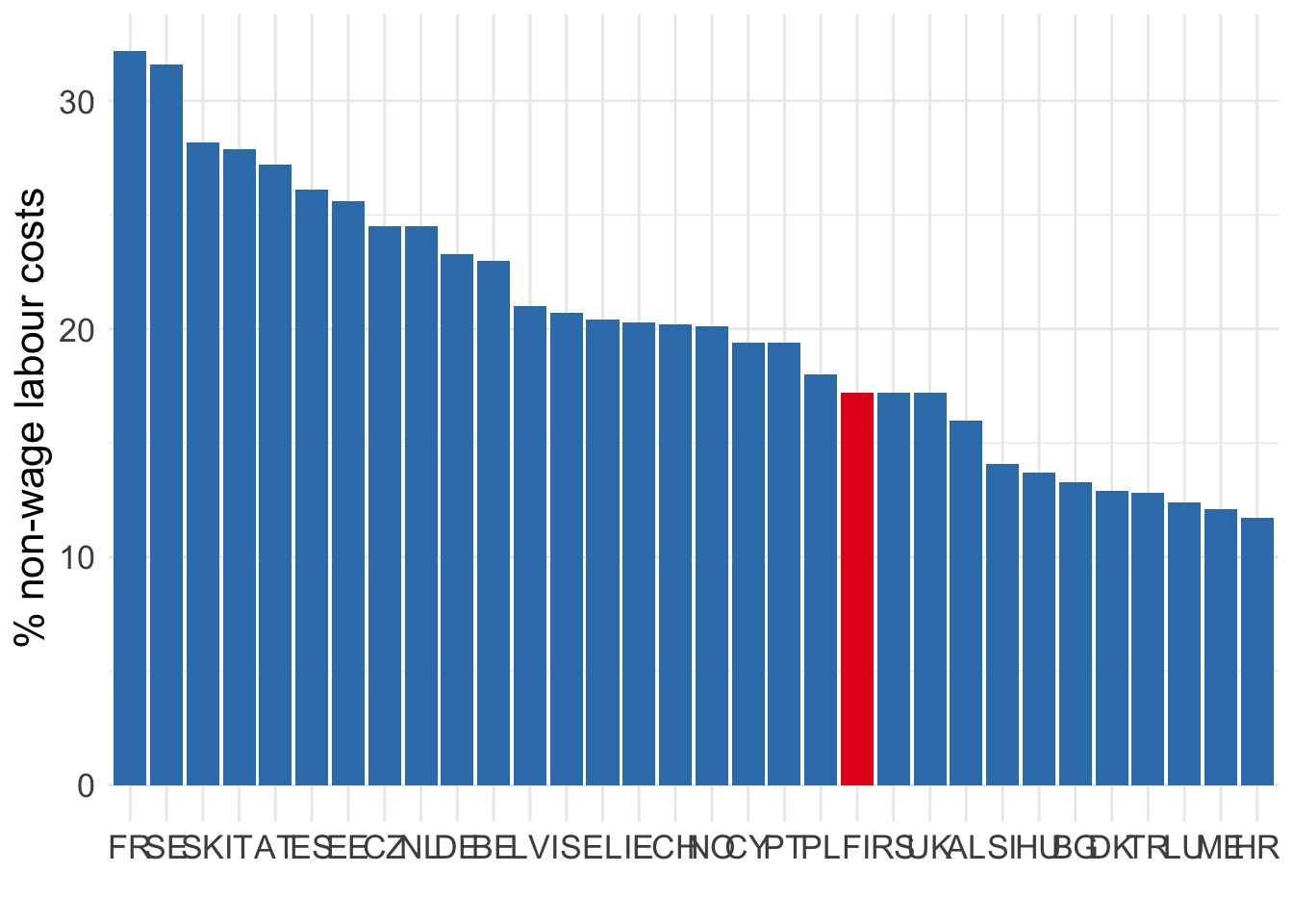
Source: Eurostat

The static models helped us analyse the optimal levels of labour demand and production in the short- and long-runs. However, they do not help us understand how do firms transition to new equilibrium points. In the static models, the assumption is that if the market conditions change, then firms can immediately shrink or expand.

In reality, adjusting employment may not be so easy for firms. Hiring new workers has costs: putting up a vacancy on a job-search portal, screening applications, interviewing candidates. The firms can pay head-hunting organizations or divert their own personnel to complete these tasks. Firing existing workers also has costs: need to give advance notice and pay wages until certain date, pay severance packages, make sure labour protection laws are not violated.

These non-wage costs of employment can be quite sizeable. According to Eurostat, non-wage labour costs account for up to 30% of total labour costs in some European countries. In Finland, share of non-wage labour costs were between 22.8% in 2008 and 17.2% in 2024. Note that these costs may also include other non-wage expenses such as occupational healthcare, travel reimbursements, lunch programs, etc.

Dynamic model

Adjustment costs

Quadratic cost: $C\left(\Delta L_t\right) = b\left(\Delta L_t - a\right)^2$
Asymmetric convex costs: $C\left(\Delta L_t\right) = -1 + e^{a\Delta L_t} - a\Delta L_t + \frac{b}{2}\left(\Delta L_t\right)^2$
Linear cost: $C\left(\Delta L_t\right) = \begin{cases}c_h \Delta L_t & \text{if }\Delta L_t \geq 0\\-c_f \Delta L_t & \text{if }\Delta L_t \leq 0\end{cases}$
Fixed cost

The simplest way to account for these non-wage costs is to specify a separate labour adjustment cost function. There are many ways you could think about these adjustment costs. We will review some of these costs in today’s lecture.

Many papers have chosen quadratic costs, which essentially means that small changes in $L$ are not as costly as very large changes in $L$.
However, the quadratic function assumes that cost of scaling up employment are identical to costs of shrinking employment, which may not be true in real life. Therefore, papers have started using asymmetric convex costs.
The functional form of asymmetric convex costs can make interpretation of model solutions complex. Therefore, some papers opted for simpler linear cost function, where slope is different for positive and negative adjustments.
These adjustment costs assume that if total employment doesn’t change $\Delta L_t = 0$, then firm does not need to pay any extra costs. But it can also be that firm hired and fired the same amount of workers. In this case, the total employment does not change, but firm still had to pay hiring costs and firing costs. To get around this issue, some papers advocate for inclusion of fixed cost of labour.

Nature of adjustment costs

Note that these adjustment costs are “weird”! You may get this impression when thinking longer about the rationale of fixed costs in adjustment costs. In these models, firms pay adjustment costs mostly when total employment changes. However, when we think about the nature of these costs, they arise at the point of hiring or firing workers.

The basic labour demand model introduced here is not suitable for studying hiring/firing decisions. Therefore, we cannot incorporate these costs separately and have to resort to more coarse proxies. In the next lecture, we will study job search models, which can be extended to include firm-side behaviour of looking for candidates. In these kinds of models, specification of hiring and firing costs is more organic.

Dynamic model

Quadratic adjustment cost

For simplicity, assume single-input: $Y_t = F(L_t)$
Continuous time: $\Delta L_t = \dot{L}_t = \frac{\text{d} L_t}{\text{d}t}$

\[ \Pi_0 = \int_0^\infty \Pi_t dt = \int_0^\infty \left[F(L_t) - W_tL_t - \frac{b}{2}\dot{L}_t^2\right]e^{-rt}~\text{d}t \]
Euler equation: $\frac{\partial \Pi_t}{\partial L} = \frac{\text{d}}{\text{d}t}\left(\frac{\partial \Pi_t}{\partial \dot{L}_t}\right)$

\[ b\ddot{L}_t - rb\dot{L}_t + F'(L_t) - W_t = 0 \]

The presence of $\dot{L}_t$ makes the derivations a little more difficult. If you are interested in the specifics, do check the textbook for derivation steps and further references!

Here, we will take Euler equation as given. It is a general result that describes the optimality condition. We can obtain expressions for the terms on the right- and left-hand sides and plug them into the Euler equation.

First, we take partial derivative of profit function at time $t$ with respect to contemporaneous level of employment $L_t$.

\[ \frac{\partial \Pi_t}{\partial L_t} = \left(F^\prime(L_t) - W_t\right)e^{-rt} \]

Next, we take partial derivative of profit function at time $t$ with respect to change in employment level $\dot{L}_t$ in the period $\text{d}t$.

\[ \frac{\partial \Pi_t}{\partial \dot{L}_t} = -b \dot{L}_t e^{-rt} \]

We can now differentiate it with respect to $t$.

\[ \frac{\partial }{\partial t}\left(\frac{\partial \Pi_t}{\partial \dot{L}_t}\right) = -b\ddot{L}_t e^{-rt} + b\dot{L}_t e^{-rt} r \]

Finally, plugging these into Euler equation we get

\[ \left(F^\prime(L_t) - W_t + b \ddot{L}_t - rb \dot{L}_t\right)e^{-rt} = 0 \]

Note that if there is no change in employment, i.e., $\dot{L}_t = \ddot{L}_t = 0$, then optimal labour supply is identical to the solution in static case.

Dynamic model

Quadratic adjustment cost

Optimal path: $\dot{L}_t = \gamma \left[L^* - L_t\right]$ where $\gamma$ is decreasing in $b$.

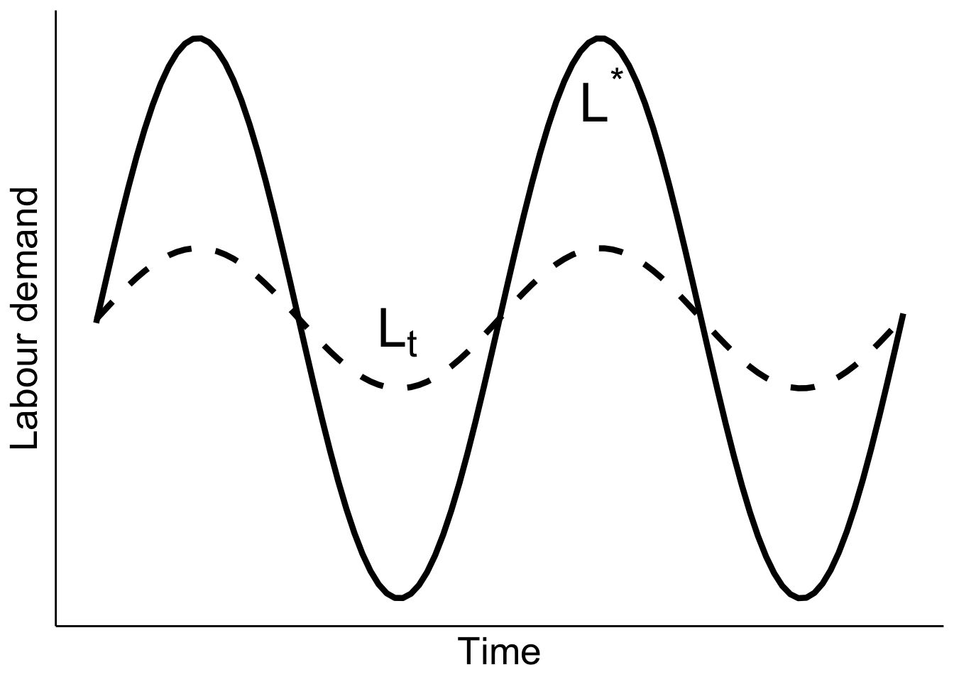
Figure 9.6 Optimal employment over a cycle (Nickell 1986)

You can denote the stationary solution $L^\star_t$ (i.e., one that satisfies $F^\prime(L^\star_t) = W_t$). The employment adjustment trajectory can be expressed as $\gamma\left[L^\star_t - L_t\right]$ with $\gamma$ decreasing in $b$ (Nickell 1986). When adjustment costs are high (high $b$), it is very costly for firms to adjust. Therefore, they will not increase or decrease labour demand $L_t$ to the full extent of the fluctuations in $L^\star_t$. In other words, the trajectory of $L_t$ will be a lot smoother than that of $L_t^\star$. What it means is that firms will not lay off all workers during recessions and not hire as many workers during booms.

In a different representation (see Figure 2.5 in Cahuc, Carcillo, and Zylberberg (2014)), it is also clear that quadratic adjustment costs imply a very long and gradual adjustment period. However, this implication is not consistent with empirical findings that show adjustments happen very quickly. And as mentioned earlier, the symmetry imposed by quadratic function can be too strong of an assumption.

Dynamic model

Linear adjustment cost

\[ \Pi_0 = \int_0^\infty \left[F(L_t) - W_tL_t - C(\dot{L}_t)\right]e^{-rt}dt \]

where $C\left(\dot{L}_t\right) = \begin{cases}c_h \dot{L}_t & \text{if }\dot{L}_t \geq 0\\-c_f \dot{L}_t & \text{if }\dot{L}_t \leq 0\end{cases}$

Optimal labour demand path is derived from

\[ \begin{cases}F'(L_t) = W_t + r c_h & \text{if }\dot{L}_t \geq 0 \\ F'(L_t) = W_t - r c_f & \text{if }\dot{L}_t < 0\end{cases} \]

Alternatively, we can specify linear adjustment costs and allow increase or decrease in employment to have different costs. Now, if labour demand increases, the firm has to pay $c_h$ for each additional unit of labour; if it decreases, the firm pays $c_f$.

The optimal labour demand is described by the two equations above. Note that $c_f > 0$ and $c_h > 0$. Therefore, there is a range of marginal products between $W_t - rc_f$ and $W_t + rc_h$ where no adjustment takes place. That is, suppose the stationary solution $L^\star_t$ varies over time within this range, then the firm will not change it’s labour demand $L_t$. However, if the stationary solution falls outside of this range, then the firm will immediately downsize or upsize its labour demand. Hence, linear adjustment costs imply sudden sharp adjustments, instead of gradual (as was the case with quadratic adjustment costs).

The linear cost function also allows us to study the changes in hiring and firing costs separately, to an extent.

Dynamic model

Linear adjustment cost

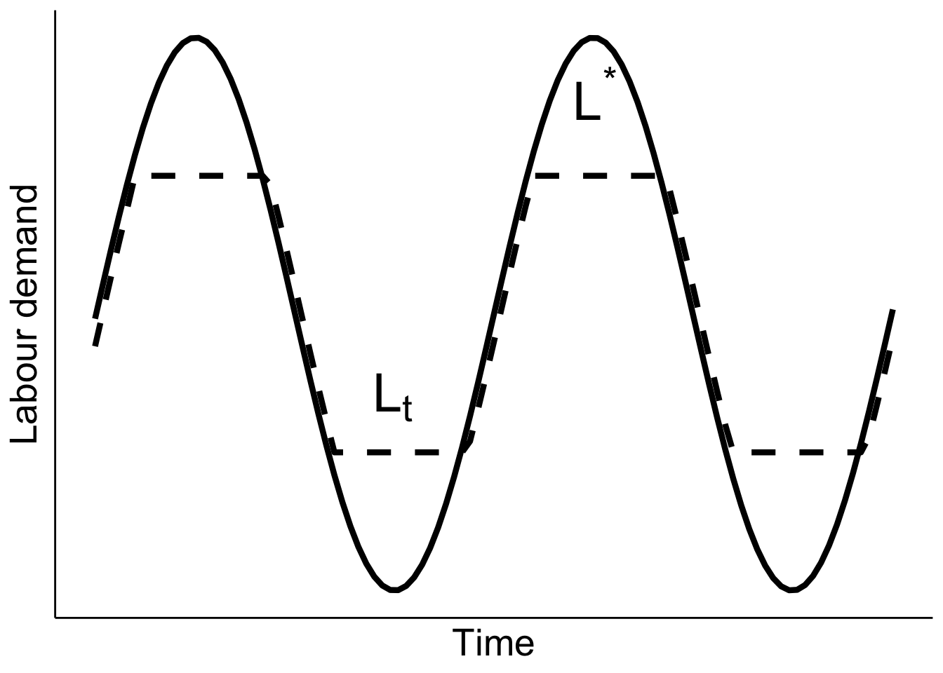
Figure 9.10 Optimal employment over the cycle (Nickell 1986)

Estimations of dynamic model

Empirical strategy for adjustment cost specification

Quadratic adjustment cost

Assume linear quadratic production function
Estimate $L_{it} = \lambda L_{i, t - 1} + X_{it} \beta + \mu_i + \varepsilon_{it}$
- Need to account for $\text{Corr}\left(L_{i, t - 1}, \mu_i + \varepsilon_{it}\right)$

A linear quadratic production function has form $F(A_t, L_t) = A_t L_t - \frac{B}{2}L_t^2$, where $A_t$ is technology of production and $L_t$ is labour input. Using this production function, quadratic adjustment costs and AR(1) process of shocks, you can derive an expression for $L_t$ as a function of $L_{t-1}$

\[ L_t = \lambda L_{t - 1} + \frac{\mu_0}{1 - \alpha(a_0 \mu_0)}a_t \]

Please check Chapter 2 in Cahuc, Carcillo, and Zylberberg (2014) for the derivations and explanation of the parameters!

This expression for the process of $L_t$ is the basis for the above regression equation. The parameter $\lambda$ depends on the adjustment costs and describes how fast the labour demand changes. Thus, if we have a panel data of firms observed over time with information about their employment levels at each point in time, we could estimate this equation.

However, notice that it cannot be estimated consistently with OLS. If you write out the equation at $t-1$, you will see clearly that the error term $\mu_i + \varepsilon_{it}$ is correlated with $L_{i, t - 1}$. You need to use appropriate dynamic panel regression methods instead.

You may also notice that this seemingly basic regression specification requires pretty strong assumptions on the functional forms of production function and labour adjustment cost function. These assumptions may not be all that justifiable.

Estimations of dynamic model

Some key results

Adjustments happen fast (1-2 quarters) (Hamermesh 1996, chap. 7)
Dynamic substitutes: utilization of capital increases with $L_t - L^*$
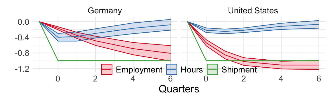
Hours of work are adjusted faster than number of workers

Figure 1 from Houseman and Abraham (1993) (adjustment to demand shocks)

Papers that study adjustment of labour and try to estimate the parameters of adjustment cost conclude that it cannot be represented by quadratic function. They suggest that most likely the shape of adjustment cost curve is piecewise linear and asymmetric. This corresponds to the case when we considered linear adjustment cost function with different slopes for employment expansion and contraction. They also suggest that the cost function should include fixed non-wage cost of labour to be consistent with the patterns observed in the data.

When they estimate speed of adjustment, the conclusion is that most of it happens really fast. Most of the adjustment takes place within 1 year and median time to adjustment is about 6 months. This is another reason why adjustment costs are unlikely to be quadratic.

Interestingly, some papers in the US find that $K$ and $L$ are dynamic substitutes. This means that when deviation of labour demand from stationary level $L_t-L^\star$ is very large, firms adjust $K$ faster. This makes sense. When the deviation of labour demand from optimal is high, the cost of adjusting the labour is at its highest. We’ve seen in the model with linear adjustment costs that in this case, firms do adjust, but only up until $L_h$ or $L_f$, which still can be very far away from optimal $L^\star$. In these cases, firms have to exploit more capital to reach the optimal production level.

Some papers have also shown that firms adjust person-hours faster than number of employees. This finding is not robustly replicated. But it can make sense since usually labour protection laws apply on the extensive margin (firing a worker) rather than on hours of work. Similarly, hiring costs apply for hiring a worker and do not vary with hours of work the person is hired for.

Also to illustrate that these costs depend on institutional context and vary greatly between countries, consider Figure 1 in Houseman and Abraham (1993). Here, the authors estimate dynamic relationships between employment in manufacturing sectors in Germany and the US, hours of work and shipments. Using the estimated coefficients, they simulate impulse response functions (IRF) of employment and hours of work following a 1-unit shock to shipments. These IRFs are plotted above. As you can see, their estimates imply that employment and hours of work fall in both countries. However, you can also see that within 2 quarters of the shock, German firms cut hours of work more severely than total employment, while the US firms layoff their workers faster than cut hours of work. This can be attributed to institutional differences in employment protection laws. In the longer run, the employment falls to the same level in Germany and the US and hours of work return to their pre-shock levels.

Note that this means adjustment patterns are estimated in the observational data. Can you think of an empirical strategy that relies on plausibly exogenous demand shocks to study this question?

For an example of a more recent paper that uses a model of labour demand with adjustment costs, see a working paper by Chan et al. (2024).

Minimum wages and employment

Minimum wage and employment

What do the models we have considered so far predict?

lower labour demand (both compensated and uncompensated)
(maybe) higher labour supply

Not always supported by empirical evidence!

The labour demand models we studied in this lecture say unequivocally that compensated and total labour demand decrease when wages rise. Therefore, if $w_\min > w^\star$ (i.e., minimum wage is above what firms would have normally paid), then labour demand should decrease.

In the last lecture, we have seen that labour supply can move in either direction depending on how strong the income effect is.

If $w^\star$ was already very high and $w^\min > w^\star$, then it is likely that income effect dominates and labour supply shrinks. In this case, total employment goes down and there are not as many unemployed individuals who should have been working without $w^\min$.
But, typically, when we think of minimum wages, we imagine that it mainly applies to situation when $w^\star$ is very low. So, then by imposing minimum wages, the government tries to ensure that all workers get some minimum decent pay. In this case, we can also hypothesise that income effect is not so strong and that total labour supply will increase when $w_\min$ is raised. In this world, we still have lower employment (because labour demand is low), but we also have a lot of unemployed people that would have been working otherwise.

However, we will see in the next slides that these predictions are not always confirmed in empirical studies.

Minimum wage and employment

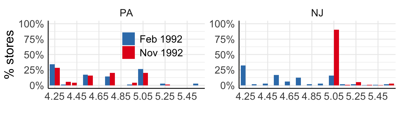
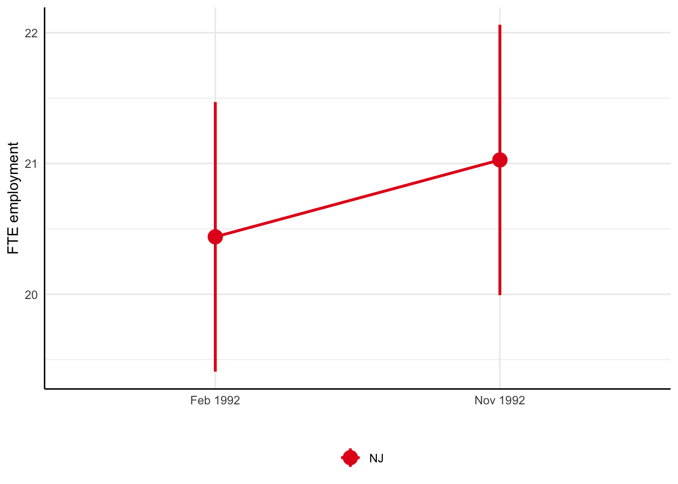
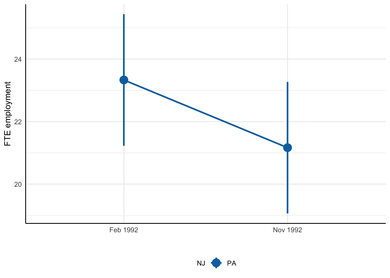
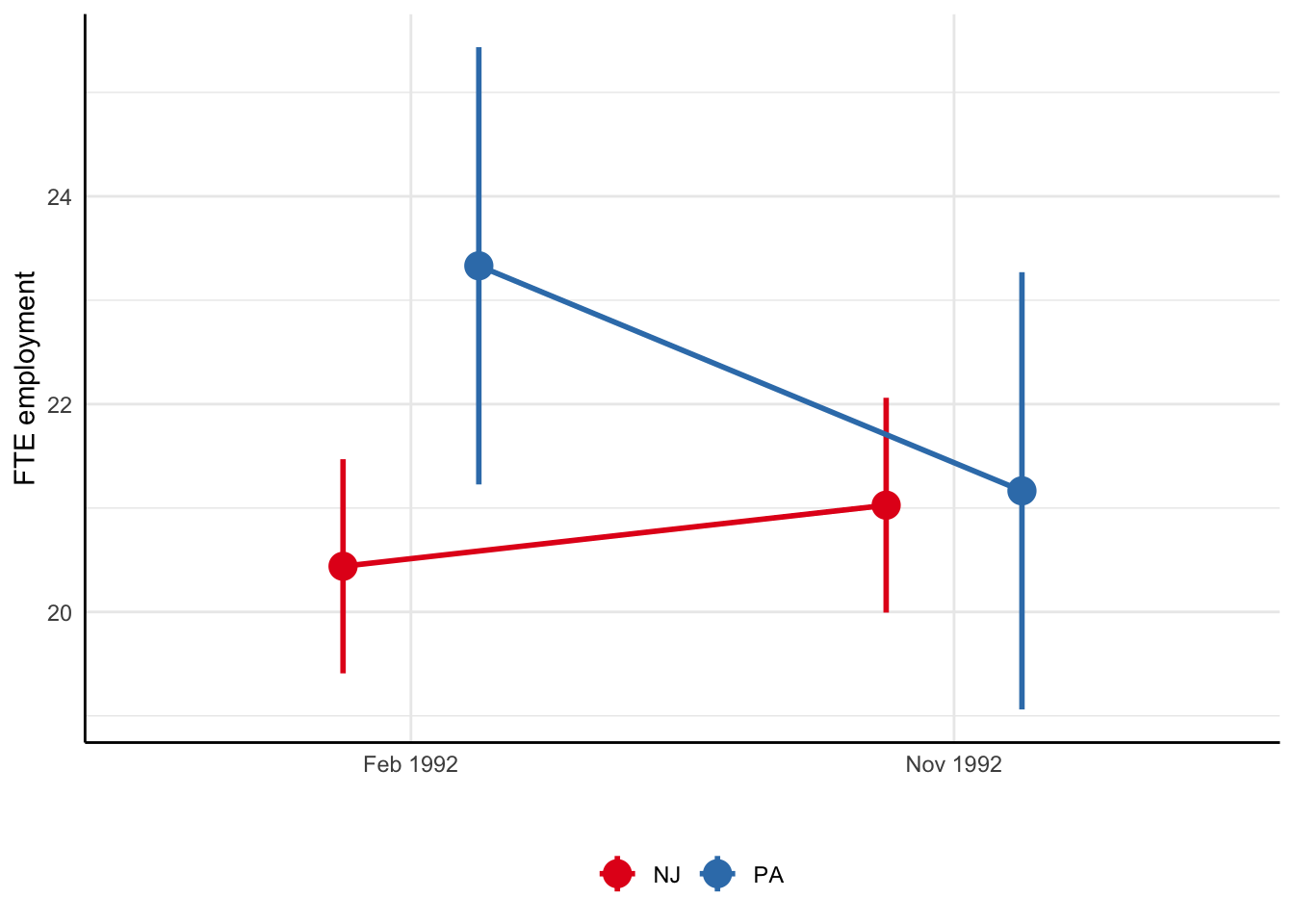
Card and Krueger (1994)

On April 1, 1992 minimum wage in New Jersey $\uparrow$ from $4.25 to $5.05.

It stayed at $4.25 in Pennsylvania.

Card and Krueger (1994) is one of the seminal papers in the field. It was among the first to use difference-in-differences estimation strategy to study the effect of a plausibly exogenous change in minimum wage law.

On 1 April 1992, the state of New Jersey increased its minimum wage level from $4.25 per hour to $5.05. At the same, the minimum wage in the neighbouring state of Pennsylvania stayed at $4.25. The authors collected data from several fast-food stores in the two states before and after the change in law. You can see in the graph above that the distribution of wages in these stores looked very similar between states before the change in the minimum wage law. After the hike, there is an increase in the number of stores in New Jersey that paid $5.05 to its workers. Also, notice that the distribution of wages in Pennsylvania did not change visibly.

The comparison over time between the states is very crucial part of the empirical strategy. If we just compare average employment in New Jersey and Pennsylvania in November 1992, we can still get biased results. We don’t know the reasons why the minimum wages were increased in one state, and not the other. It could be that general level of wages rose sufficiently fast in NJ so that higher minimum wage would still be below the equilibrium wage, whereas in PA wages weren’t rising as fast. In short, there may be some systematic differences between NJ and PA that would correlated both with their labour markets and with the probability that one state increases its minimum wage, while other doesn’t. Since this policy was not implemented in a randomised manner, we cannot rule out the existence of such systematic difference. Therefore, if we just compared the variables in two states in November 1992, we would pick up on those differences in addition to the causal effect of minimum wages.

Alternatively, you might think that you could focus on fast-food stores in New Jersey alone and simply compare their outcomes before and after the policy change. That is, you can compute average outcome of NJ stores in November 1992 and April 1992 and take their difference. In this case, the difference over time will also pick up some time trend in addition to the causal effect of minimum wages. In other words, there are other reasons for average wages or employment to change over time besides the policy change. Often, wages are indexed to inflation and grow over time. Here, especially, you may also pick up on seasonal patterns of wages. Employment too can follow time trends (for example, due to business cycles) and seasonal patterns.

However, you could use change in average outcomes over time in Pennsylvania as a proxy for time trends in New Jersey. This is why the estimation is called difference-in-differences: you take difference over time in each state and then subtract one time difference from another. You will see it clearly in the next slide.

Minimum wage and employment

Card and Krueger (1994): Difference-in-differences

Compare before and after in NJ:
$E_{t1}^{NJ} - E_{t0}^{NJ}$ = 0.59 (se = 0.73)

Minimum wage and employment

Card and Krueger (1994): Difference-in-differences

Compare before and after in NJ:
$E_{t1}^{NJ} - E_{t0}^{NJ}$ = 0.59 (se = 0.73)
Compare before and after in PA:
$E_{t}^{NJ} - E_{t}^{PA}$ = -2.17 (se = 1.65)

Minimum wage and employment

Card and Krueger (1994): Difference-in-differences

Compare before and after in NJ:
$E_{t1}^{NJ} - E_{t0}^{NJ}$ = 0.59 (se = 0.73)
Compare before and after in PA:
$E_{t}^{NJ} - E_{t}^{PA}$ = -2.17 (se = 1.65)
Diff-in-diff:
$\left(E_{t1}^{NJ} - E_{t0}^{NJ}\right) - \left(E_{t1}^{PA} - E_{t0}^{PA}\right)$ = 2.75 (se = 1.69)

Therefore, you can clearly see that the difference-in-differences estimator of the causal effect is positive. That is, an increase of minimum wage from $4.25 to $5.05 has increased average employment in New Jersey by 2.75 workers. This corresponds to 18.8% rise in minimum wages and 13.5% increase in average employment. The implied elasticity, therefore, is 0.7. However, note that standard errors are very high and we cannot reject the null hypothesis for any of these differences.

Maybe at this point you feel a little confused: how could such a fundamental prediction of basic labour models be so wrong? I encourage you to think about these results closely.

What do you think could explain the opposite sign of employment response?
Do you think the estimation strategy might still be overlooking something?

Try to answer these questions and think about what could be done to improve the estimates!

Minimum wage and employment

Jardim et al. (2022)

Seattle $\uparrow$ min wage from $9.47 up to

$11 in April 2015
$13 in January 2016

Causal design:

synthetic control: weighted average of other counties match pre-Seattle
nearest neighbour matching: find “closest” worker outside of Seattle matching treated worker in Seattle

As it turns out, not all economists agree with the result of Card and Krueger (1994). And you might be surprised that the debate about the effect of minimum wages is alive to this day. Here is another a more recent paper by Jardim et al. (2022) that studies a similar change in policy. The minimum wages in Seattle were raised first from $9.47 to $11 in April 2015 and then to $13 in January 2016.

Instead of comparing Seattle to the nearest state or municipality, the authors here adopt a so-called synthetic control estimation strategy. Think back to Card and Krueger (1994). The identification implicitly assumes that stores in NJ and PA would have similar time trends. This is called parallel trends assumption. If NJ did not increase its minimum wages, then average employment in NJ would also decrease by similar amount as average employment in PA. But there may be some differences between the states that we cannot account for that might make this assumption invalid. On top of it, why should we rely on PA alone when there might be other states that would have similar time trends?

The synthetic control does not use just one group of controls (for example, stores in nearest municipality to Seattle), but, as the name suggest, generate synthetic control from average employment in many plausibly similar groups (municipalities). Imagine that municipality of Helsinki introduced minimum wages. You could use maybe municipality of Espoo as control group (assuming they did not implement minimum wages), or you could use average employment in Espoo, Vantaa and Tampere to construct “synthetic Helsinki” without minimum wages.

The second approach Jardim et al. (2022) is to match workers from Seattle to similar workers outside of Seattle using nearest neighbour matching. Similar to the reasoning before, just comparing workers in Seattle and outside will contain not only causal effect of minimum wages, but also all other differences between workers in different locations. Maybe Seattle is particularly interesting for certain industry and it is hard to find similar jobs outside of Seattle. Maybe there are more career opportunities in Seattle compared to other places. By matching workers, the authors attempt to find the most observationally similar workers. They need to be of similar age, similar educational background, maybe even hold similar jobs and work in similar industries before April 2015. This way you can compare these workers and attribute any differences between them to the effect of policy change.

Minimum wage and employment

Jardim et al. (2022): synthetic control

The graphs above show the results from synthetic control estimations on average wages, employment and hours of work. These are basically differences in average outcomes in Seattle from average outcomes in synthetic control group plotted over time. The two vertical lines mark April 2015 and January 2016, two episodes of minimum wage hikes in Seattle.

First of all, average wages go up. This is mechanical effect since firms in Seattle cannot pay wages below new minimum wage levels.

Second, you can see mildly negative impact on employment and hours of work. But we cannot reject the null hypothesis that these effects are zero. Even though there doesn’t seem to be a clear, strong reduction in labour demand, these results are more in line with standard labour theories.

Another interesting exercise the authors do in this paper is that they look at the effect throughout the wage distribution. In the graph above, the authors focus on workers that were paid less than $19 before the policy change. These are the workers most likely to have been affected directly by the minimum wage laws.

The theories of labour demand and labour supply we have seen so far do not generate distribution of wages. So, it is difficult to make informed predictions of how should minimum wages affect wages and employment of workers higher up in the distribution. But we can guess that there might be an upward pressure on wages above $19 as well. It could be that firms decide to substitute partially away from minimum wage workers to more skilled workers. Higher demand, higher wage. It could be that non-minimum wage workers are able to negotiate higher salaries because higher minimum wage gives them a little more bargaining power. What can then happen to employment of non-minimum-wage workers? On the one hand, their labour supply may increase in response to higher wages. On the other hand, firms may decide to shrink production and reduce overall labour demand.

Minimum wage and employment

Jardim et al. (2022): synthetic control

In the graph above, Jardim et al. (2022) show average outcomes of workers that were earning more than $40 before the policy change. These workers are not directly affected by the minimum wage law, but can experience indirect effects as discussed earlier.

Notice that average wages of high-earners also goes up after minimum wages rose. Moreover, wages of high-earners response a lot more strongly! The authors also report mildly positive impact on employment and hours of work among high-earning workers.

However, this result can add a grain of salt to the overall findings. Why do the outcomes of high-earning workers respond so strongly? Can it be that Seattle economy was developing in a way that a sizeable shift from low- to high-paying jobs occurred simultaneously with an increase in minimum wages? If so, then the estimation results remain biased.

Finally, if you read the paper more closely, you will notice that the authors have excluded firms that operate in multiple locations. Moreover, these firms account for about 40% of Seattle’s low-wage employment! Can you think of reasons why such seemingly innocuous sample selection criterion can change the results?

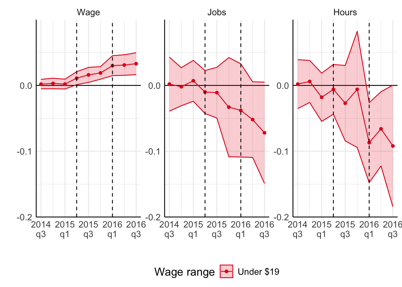
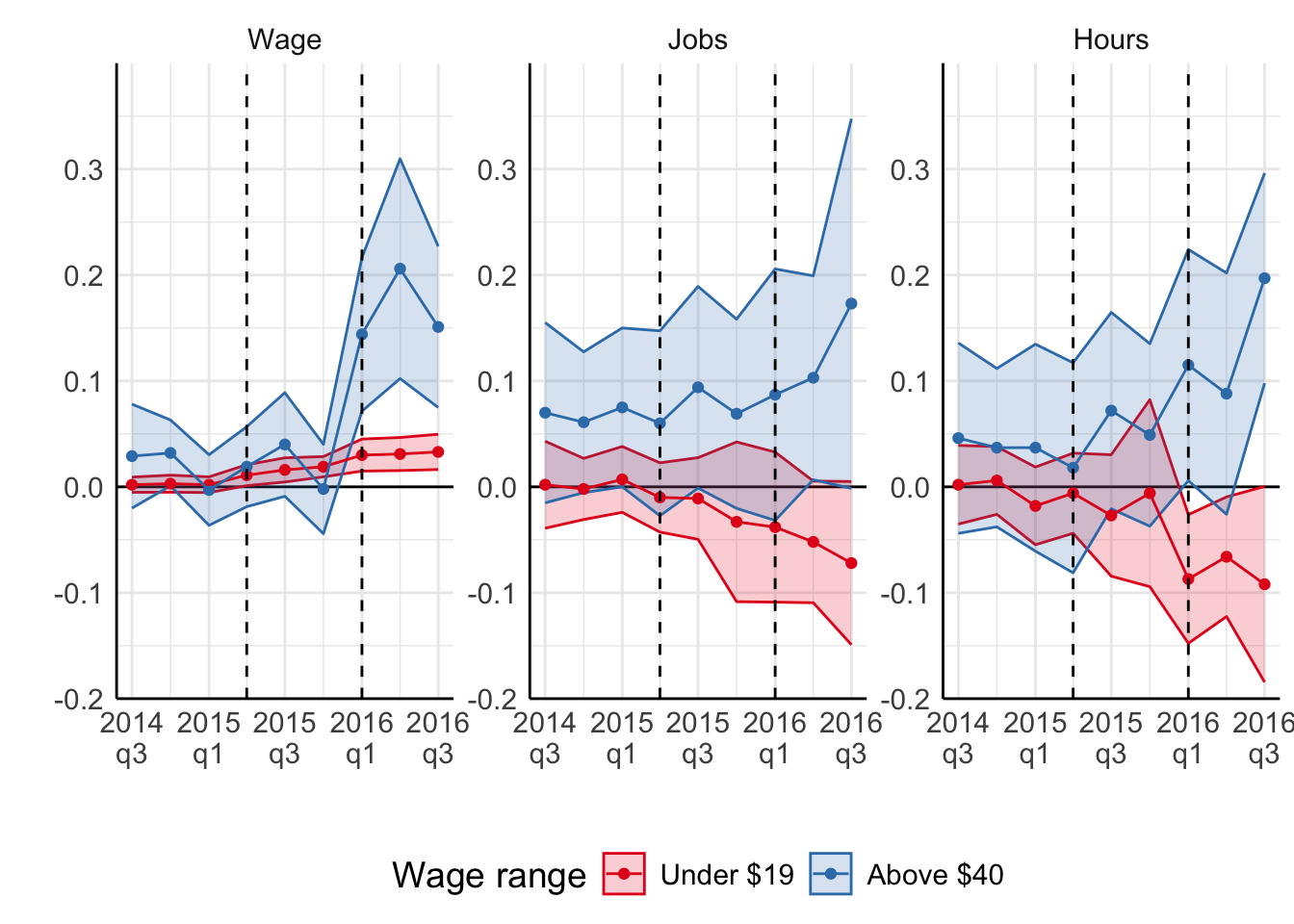
Minimum wage and employment

Jardim et al. (2022)

Negative effect on hours worked stronger than on employment
Experienced workers are better off

However,

Potentially cascading effect
Excluded large low-wage employers (like McDonald’s)

Reich, Allegretto, and Goddy (2017)

same policy + synthetic control = no change in employment

Minimum wage and other margins

Review in Clemens (2021)

Price pass-through (Leung 2021; Renkin, Montialoux, and Siegenthaler 2022)
Non-wage labour cost (Clemens, Kahn, and Meer 2018)
Flexibility (theoretical Clemens and Strain 2020)
Effort (Ku 2022; Coviello, Deserranno, and Persico 2022)
Firm profit (Draca, Machin, and Van Reenen 2011; Bell and Machin 2018)
Firm exit (Luca and Luca 2019; Dustmann et al. 2022)

So, if we believe that raising minimum wages does not have a significant impact on employment and labour demand, how could we explain it? There are several possible mechanisms that have been examined in the literature.

Price pass-through.

Firms that employ minimum-wage workers and that now have to pay them higher wages, may simply increase their prices. Thus, they pass the higher wage costs onto the consumers. Note that this explanation can only work with imperfect competition in the product market. If there was perfect competition, then firm would have been unable to raise its prices. For example, the firm may be a monopoly, so consumers have no alternative to turn to. Or, consumers do not look around for better prices, as long as price increases are not too drastic.
Non-wage labour cost.

Recall earlier discussion that firms pay wage and non-wage costs for labour. These non-wage costs can include many different benefits such as occupational healthcare. The non-wage costs are rarely regulated. Therefore, firms have more freedom in adjusting these costs compared to wages or changes in employment. For example, they may decide to decrease healthcare coverage or stop providing lunch benefits following an increase in wages.
Flexibility.

Another interesting channel is work flexibility. Clemens and Strain (2020) provide a stylised discussion of this channel, albeit not estimated using any data. In their framework, the consumer demand is not constant: there are periods of time when it is high or low. This can, for example, be very reasonable description of the demand in restaurants. Firms can choose flexibility of employment conracts. For example, they can hire waiters to come every day from 10 to 18, or they can call the waiters only when demand is high. In the first case, they have to pay wages to the waiters regardless of whether there were customers in the restaurant or not. In the second case, the restaurant would only call its waiters when there are customers and pay them only for the actual number of hours worked. The authors suggest that when wages increase, firms might favour such irregular contracts more.
Effort.

There’s been quite a few recent papers that try to quantify the response in effort of work following a minimum wage hike. You can imagine that firms that have to pay higher wages would have higher requirements and give their workers more (or more difficult) tasks. Thus, workers might keep their jobs, but need to work harder after minimum wage increases.
Firm profit.

It might simply be that the firm decides to finance higher wages out of its own profit. This might be the case in the short-run (many papers that study effect of minimum wages look at rather short windows of time) and in the presence of adjustment costs.

What do you think might happen in the longer run?
Firm exit.

Finally, firms might just find it too expensive to operate and decide to close down.

Whatever the reason, these considerations alone highlight that decisions that firms can and do make are more complicated than simply choosing $L$, $K$ and $Y$. In the past these kinds of questions were difficult to answer due to lack of appropriate data. Nowadays, high-quality firm-level data is more available and covers larger set of firm characteristics and outcomes. These and many other questions become feasible to study empirically! For example, see a working paper by Elias and Riudavets-Barcons (2024) for the study of the impact of minimum wages on collective bargaining agreements.

We will see, at least references, to some of these channels in the next two lectures.

Summary

Basic static and dynamic models of labour demand
Application to minimum wage policy
- Ongoing research (little consensus)
- Clear that basic models are insufficient
- Non-wage margins important and can interact with labour supply

Next lecture: Job Search on 03 Sep

References

Bell, Brian, and Stephen Machin. 2018. “Minimum Wages and Firm Value.” Journal of Labor Economics 36 (1): 159–95. https://doi.org/10.1086/693870.

Cahuc, Pierre. 2004. Labor Economics. Cambridge (Mass.): MIT Press.

Cahuc, Pierre, Stéphane Carcillo, and André Zylberberg. 2014. Labor Economics. Second edition. Cambridge, MA: The MIT Press. https://research.ebsco.com/linkprocessor/plink?id=0949c8a9-3435-3a85-a9e3-d47d2c8a57ef.

Card, David, and Alan B. Krueger. 1994. “Minimum Wages and Employment: A Case Study of the Fast-Food Industry in New Jersey and Pennsylvania.” The American Economic Review 84 (4): 772–93. https://www.jstor.org/stable/2118030.

Chan, Mons, Elena Mattana, Sergio Salgado, and Ming Xu. 2024. “Dynamic Wage Setting: The Role of Monopsony Power and Adjustment Costs.” February 15, 2024. https://www.monschan.com/papers/CMSX_2024_BSF.pdf.

Clemens, Jeffrey. 2021. “How Do Firms Respond to Minimum Wage Increases? Understanding the Relevance of Non-Employment Margins.” Journal of Economic Perspectives 35 (1): 51–72. https://doi.org/10.1257/jep.35.1.51.

Clemens, Jeffrey, Lisa B. Kahn, and Jonathan Meer. 2018. “The Minimum Wage, Fringe Benefits, and Worker Welfare.” NBER Working Paper. Working Paper Series. May 2018. https://doi.org/10.3386/w24635.

Clemens, Jeffrey, and Michael R. Strain. 2020. “Implications of Schedule Irregularity as a Minimum Wage Response Margin.” Applied Economics Letters 27 (20): 1691–94. https://doi.org/10.1080/13504851.2020.1713978.

Coviello, Decio, Erika Deserranno, and Nicola Persico. 2022. “Minimum Wage and Individual Worker Productivity: Evidence from a Large US Retailer.” Journal of Political Economy 130 (9): 2315–60. https://doi.org/10.1086/720397.

Draca, Mirko, Stephen Machin, and John Van Reenen. 2011. “Minimum Wages and Firm Profitability.” American Economic Journal: Applied Economics 3 (1): 129–51. https://doi.org/10.1257/app.3.1.129.

Dustmann, Christian, Attila Lindner, Uta Schönberg, Matthias Umkehrer, and Philipp vom Berge. 2022. “Reallocation Effects of the Minimum Wage*.” The Quarterly Journal of Economics 137 (1): 267–328. https://doi.org/10.1093/qje/qjab028.

Elias, Ferran, and Marc Riudavets-Barcons. 2024. “The Interaction Between Minimum Wages and Collective Bargaining: Explaining Wage Spillovers.” November 10, 2024. https://drive.google.com/file/d/1tMntO_HARfY34vKJD68rx0iCWb9gr6UW/view?usp=sharing&usp=embed_facebook.

Hamermesh, Daniel S. 1996. Labor Demand. Princeton University Press.

Houseman, Susan N, and Katharine G Abraham. 1993. “Labor Adjustment Under Different Institutional Structures: A Case Study of Germany and the United States.” NBER Working Paper 4548. Cambridge, MA. October 1993. https://www.nber.org/system/files/working_papers/w4548/w4548.pdf.

Jardim, Ekaterina, Mark C. Long, Robert Plotnick, Emma van Inwegen, Jacob Vigdor, and Hilary Wething. 2022. “Minimum-Wage Increases and Low-Wage Employment: Evidence from Seattle.” American Economic Journal: Economic Policy 14 (2): 263–314. https://doi.org/10.1257/pol.20180578.

Ku, Hyejin. 2022. “Does Minimum Wage Increase Labor Productivity? Evidence from Piece Rate Workers.” Journal of Labor Economics 40 (2): 325–59. https://doi.org/10.1086/716347.

Leung, Justin H. 2021. “Minimum Wage and Real Wage Inequality: Evidence from Pass-Through to Retail Prices.” The Review of Economics and Statistics 103 (4): 754–69. https://doi.org/10.1162/rest_a_00915.

Luca, Dara Lee, and Michael Luca. 2019. “Survival of the Fittest: The Impact of the Minimum Wage on Firm Exit.” NBER Working Paper. Working Paper Series. May 2019. https://doi.org/10.3386/w25806.

Nickell, S. J. 1986. “Chapter 9 Dynamic Models of Labour Demand.” In Handbook of Labor Economics, 1:473–522. Elsevier. https://doi.org/10.1016/S1573-4463(86)01012-X.

Reich, Michael, Sylvia Allegretto, and Anna Goddy. 2017. “Seattle’s Minimum Wage Experience 2015-16.” SSRN Electronic Journal. https://doi.org/10.2139/ssrn.3043388.

Renkin, Tobias, Claire Montialoux, and Michael Siegenthaler. 2022. “The Pass-Through of Minimum Wages into U.S. Retail Prices: Evidence from Supermarket Scanner Data.” The Review of Economics and Statistics 104 (5): 890–908. https://doi.org/10.1162/rest_a_00981.