2. Labour Supply

KAT.TAL.322 Advanced Course in Labour Economics

Nurfatima Jandarova

August 27, 2025

Today

• Static model
• Household model
• Intertemporal model
• Estimations

Labour supply

How people choose

• whether to work, and
• how much to work

Static model

Static labour supply

Model

• Utility from consumption of goods (\(C\)) and leisure (\(L\)): \(U(C, L)\).
• Total time endowment \(L_0\)
• Agent chooses \(h\) how much time to work such that \(L = L_0 - h\).
• Budget constraint is \(C \leq wh + Y \Rightarrow C + w L \leq w L_0 + Y\)
  • \(w\) is real hourly wage
  • \(Y\) is non-labour income

\[ \max_{C, h} U(C, L_0 - h) \quad\text{subject to} \quad C \leq wh + Y \]

• In economics, the tradeoffs arise from finite resources. Hence, we need to find the best way to allocate that finite resource.
• In the case of a worker making decisions, the finite resource is her time (\(L_0\)).
• The individual can devote all her time to working to maximise earnings. But that clearly is undesirable because she would then not enjoy any recreation time and will not be performing other every day activities (home production).
• She could also devote all her time to leisure and home production. That too would be undesirable because these activities do not earn wages, so she would not be able to consume much.
• So, she needs to find an optimal time she wants to devote to work \(h\) such that she has enough income to finance her consumption and enough time for leisure and home production.
• This is the most standard model of labour supply used as the basis for many other extensions (such as wealth accumulation, occupation choice, family formation, even criminal activity). Despite its simplicity, it can illustrate the tradeoffs well and inform our interpretation of the real world.

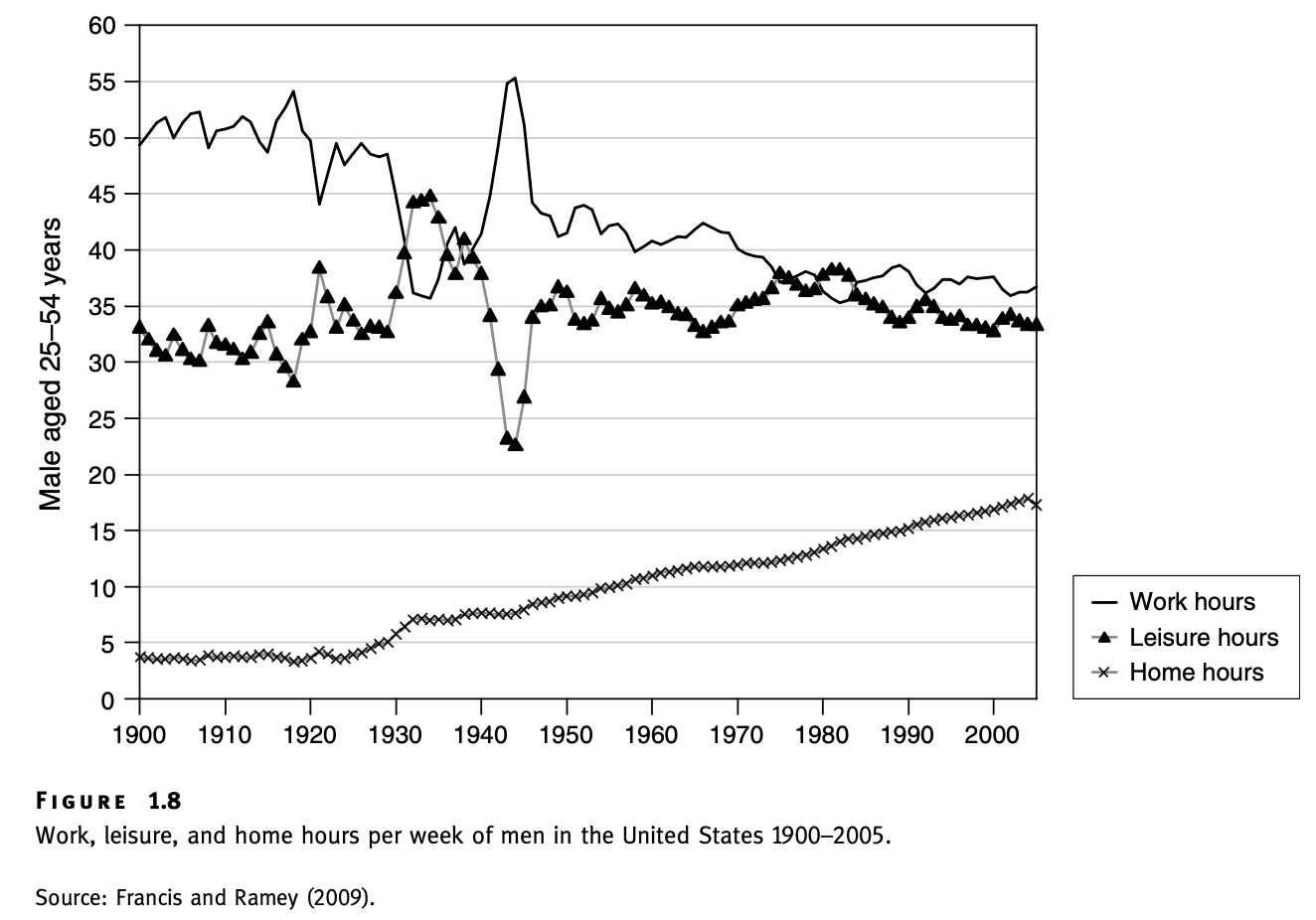
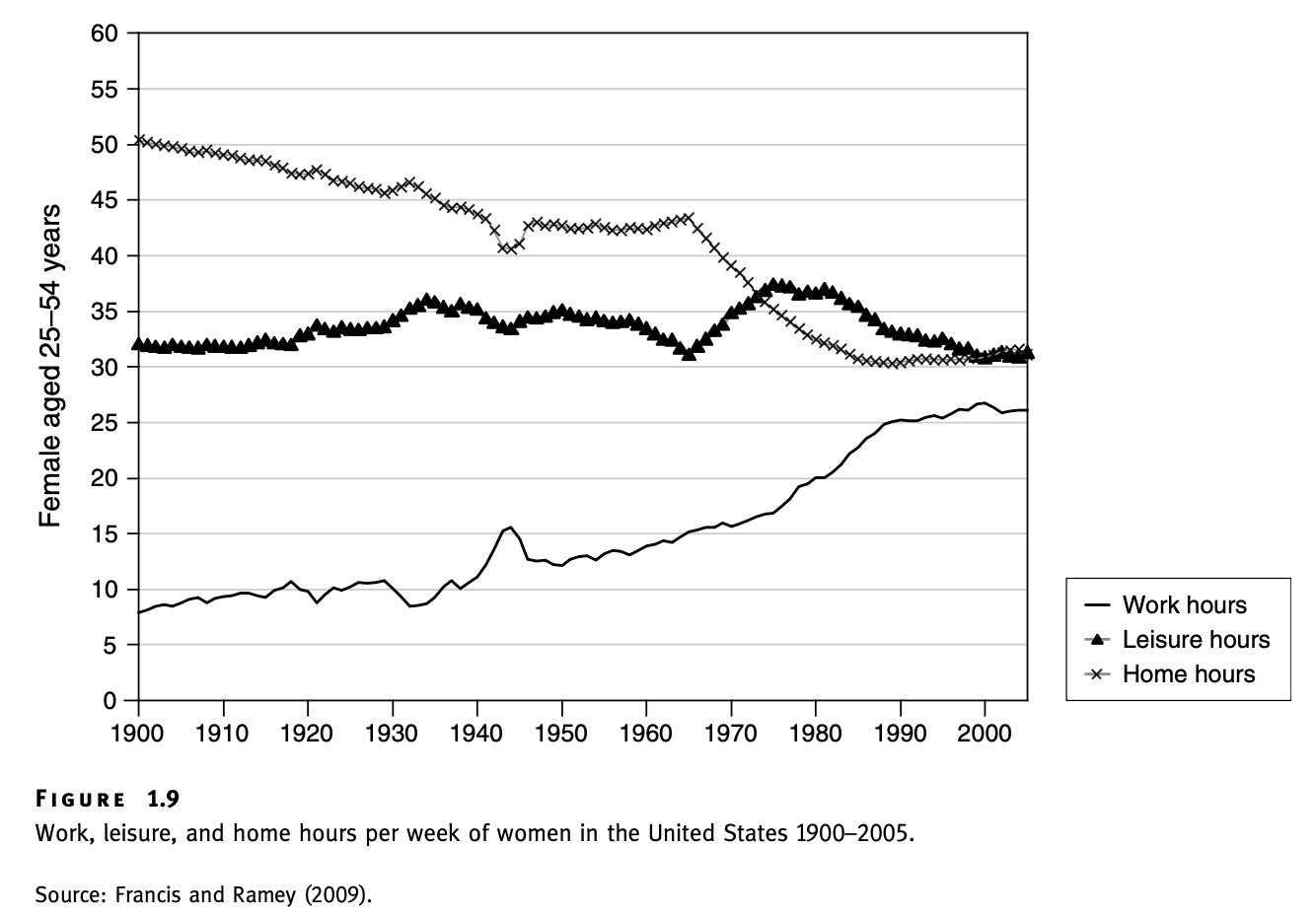
Static labour supply

Allocation of time in the data

Men

Women

Ramey and Francis (2009) study the evolution of average work, leisure and home production hours throughout the XX century.

• Work hours have increased markedly for women and declined for men.
• However, total number of hours devoted to work has declined slightly over the same years (see figure in Ramey and Francis (2009)).
• Despite this the leisure hours have not changed much.
• Instead, the dynamics in work hours seem to be reflected in the dynamics of the home production hours: women have decreased time devoted to home production, while men increased.
• The change seems to be symmetric so that the total amount of time spent on home production across both sexes remained roughly similar over the years.
• There was also noticeable increase in the time spent on education (not shown in the graphs).

Static labour supply

Solution

First-order conditions of the Lagrangian are

\[ U_C(C, L) = \lambda \qquad U_L(C, L) = \lambda w \]

Solution pair \(C^*(w, Y)\) and \(h^*(w, Y)\) satisfies

\[ \frac{U_L(C^*, L^*)}{U_C(C^*, L^*)} = w \quad \text{and} \quad C^* = wh^* + Y \]

Typical way to solve constrained optimisation problem is to set up a Lagrangean.

\[ L = U(C, L_0 - h) + \lambda\left(Y + wh - C\right) \]

Now, we can take first-order derivaties with respect to \(C\) and \(h\) and equate them to zero (equivalent to finding a tangency point between indifference curve and budget line).

\[ \frac{\partial L}{\partial C} = U_C(C^\star, L_0 - h^\star) - \lambda = 0 \]

\[ \frac{\partial L}{\partial h} = -U_L(C^\star, L_0 - h^\star) + \lambda w = 0 \]

Hence, first-order conditions (FOCs) are as presented on the slide. We can now divide the two FOCs to get the optimality condition

\[ \frac{U_L(C^*, L_0 - h^*)}{U_C(C^*, L_0 - h^*)} = w \]

Static labour supply

Solution

The solution can be depicted graphically in the \(C\)-\(L\) space.

• The straight line is the budget line: it traces all combinations of \(C\) and \(L\) that can be accommodated with the same budget (given \(w\) and \(Y\))
• The curve is indifference curve: it traces all combinations of \(C\) and \(L\) that deliver same level of utility \(U\)
• The optimal solution lies at the point of tangency of two curves: the combination of \(C\) and \(L\) that gives highest utility, while still being feasible.

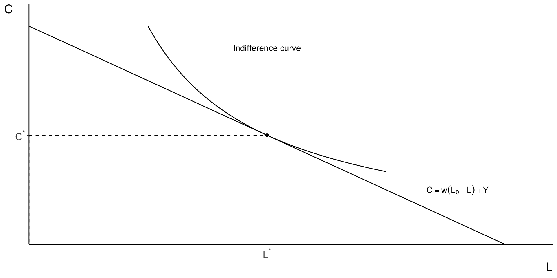
Static labour supply

Comparative statics

How does optimal labour supply change with \(w\)?

Marshallian (uncompensated) wage elasticity: \(\varepsilon_{hw} = \frac{\partial \ln h^*}{\partial \ln w}\)

Hicksian (compensated) wage elasticity: \(\eta_{hw} = \frac{\partial \ln \hat{h}}{\partial \ln w}\)

Decomposition into substitution and income effects:

\[ \varepsilon_{hw} = \color{#8e2f1f}{\eta_{hw}} + \color{#288393}{\frac{wh}{Y} \varepsilon_{hY}} \]

Given the solution of the simple static model, we can form predictions about labour supply. In particular, we can evaluate how does optimal labour \(h^\star\) vary with \(w\) and \(Y\).

The first kind of elasticity is called Marshallian elasticity. We can easily find it by differentiating the optimal solution \(h^\star(w, Y)\) with respect to \(w\). This will give us total change in the optimal labour supply.

However, the total change in labour supply comes from two sources. When \(w \uparrow\), the opportunity cost of leisure goes up. That is, every hour that she’s not working, she is foregoing the opportunity of earning higher \(w\). Therefore, the worker has higher incentive for increasing her labour supply \(h\). This is called substitution effect.

At the same time, now that she’s earning higher \(w\) for every hour spent working, she is also enjoying higher overall income \(wh + Y\). Conversely, she can decrease her labour supply \(h\) (and increase her leisure \(L\)) and still maintain same budget as before \(w\) rose. This is called income effect.

The Hicksian elasticity is crucial part of the decomposition of these two effects. If you recall, the duality principle allows you to solve optimisation problems by either

• maximising utility holding budget constant, or
• minimising expenditure holding utility constant.

If you solve the dual of the original optimisation problem, you will get optimal solution \(h^\star(w, \bar{U})\) and \(C^\star(w, \bar{U})\). You can then derive Hicksian elasticity by differentiating \(h^\star(w, \bar{U})\) with respect to \(w\). Since it fixes the utility at \(\bar{U}\), this elasticity only captures the substitution effect.

The decomposition of Marshallian elasticity into substitution and income effect is known as Slutsky equation.

Despite the simplicity, knowing these elasticities can be useful tools. For example, if you need to quickly assess implications of some labour policy or some external shock to wages.

Static labour supply

Comparative statics

Source: Wikipedia

The idea behind the substitution and income effects can also be presented graphically.

• We star of at point \(A\).
• There is a policy change that increases wages \(w\). As a result, the budget line rotates outwardly.
• The new optimal solution lies at point \(B\).
• Thus, the change from \(A\) to \(B\) will capture total Marshallian elasticity.
• However, notice that the indifference curve \(IC_2\) could have been reached under the old \(w\), if non-wage income \(Y\) were just higher. If this were the case, the optimal point would have been at point \(C\).
• Hence, change from \(A\) to \(C\) captures income elasticity of labour supply.
• Now, the idea behind Hicksian elasticity is we hold utility, or indifference curve, constant. That is, now we simply rotate the budget line to match new \(w\) and get point \(B\).
• Therefore, change from \(C\) to \(B\) captures the substitution effect.

Static labour supply

Labour supply curve

Source: Wikipedia

Because of the income effect, the labour supply curve may not always be increasing in wage \(w\).

• Suppose we started at point \(E\) and kept increasing wage \(w\).
• The previous analysis shows that the overall change in \(h^\star\) is a combination of substitution and income effects.
• It is likely that at low values of \(w\), substitution effect prevails and the worker increases her labour supply with \(w\).
• However, once we reach point \(F\), wages are now so high that increasing them further would make sure that income effect prevails. Hence, overall labour supply would start falling if wages continue rising.

Household model

Intrahousehold labour supply

Unitary model

Household represented by single utility function \(U(C, L_1, L_2)\)

Budget constraint \(C + w_1 L_1 + w_2 L_2 \leq Y_1 + Y_2 + (w_1 + w_2) L_0\)

• Simple extension of static model

• Consumption depends on total resources only

• Not consistent with empirical studies

The simple static model assumes a household with a single member. However, this is not always true: households often consist of multiple members who decide on their labour supply simultaneously. Thus, their optimal decisions may depend on each other.

In this model, we have two agents with own wage rates \(w_1\) and \(w_2\) that need to decide on their respective labour supply \(L_1\) and \(L_2\). Consumption happens at the household level and depends on overall resources, including non-wage income of both members, \(Y_1\) and \(Y_2\). In addition, the utility of the household remains unitary.

This is simplest form of extension, since optimal solutions only depend on total income \(Y_1+Y_2\). So, if members 1 and 2 are husband and wife, it doesn’t matter for the total consumption whether higher non-wage income comes from husband or wife. However, many empirical studies have found evidence to the contrary: distribution of \(Y_1\) and \(Y_2\) can also matter¹.

1. Lundberg, Pollak, and Wales (1997) show that paying child benefits to mothers’ accounts instead of father’s increases the share of household consumption on women’s and children’s goods.

Intrahousehold labour supply

Collective model

Individual utility functions \(U_1(C_1, L_1), U_2(C_2, L_2)\)

Budget constraint \(C_1 + C_2 + w_1 L_1 + w_2 L_2 \leq R_1 + R_2 + (w_1 + w_2) L_0\)

\[\begin{align} \max_{C_1, C_2, L_1, L_2} U_1(C_1, L_1) \quad\text{s.t.}\quad&\text{budget constraint}\\ & U_2(C_2, L_2) \geq \bar{U}_2 \end{align}\]

In the collective version

• the division of total resources may not be equal and is captures by \(\mathbf{\Phi}_i\)
• each member may have her own utility function \(U_1(\cdot)\) and \(U_2(\cdot)\)

The optimal solution can be found by maximising the utility of one of the members subject to the budget constraint and utility level of the other member. This is called partner utility constraint and ensures that optimal solution conforms to the idea of Pareto efficiency. That is, optimal solution is such that one member cannot be made any more happier without hurting the other.

Intrahousehold labour supply

Collective model

Chiappori (1992): equivalent to

\[ \max_{C_i, L_i} U_i(C_i, L_i) \quad\text{s.t.}\quad C_i + w_i L_i \leq w_i L_0 + \Phi_i \]

where \(\Phi_i\) describes how resources \(R_1 + R_2\) are shared in the household.

According to Chiappori (1992), the same optimal solution can be achieved by having each household member solve their own individual optimisation problems with a slight adjustment to their budget constraint. Instead of having their own non-earned income \(Y_i\), their budget, instead, depends on the division of total household income \(\mathbf{\Phi}_i\).

You can try solve either version of this extension and derive the comparative statics. What can you say about labour supply of household members with respect to their own wages? With respect to their spouse’s wage?

For more, see (Cahuc 2004, chap. 1) and Chiappori (1992)

Intertemporal model

Intertemporal labour supply

Model

General utility function \(U(C_0, \ldots, C_T; L_0, \ldots, L_T)\) (intractable)

Separable utility function \(\sum_{t = 0}^T U(C_t, L_t, t)\)

Budget constraint \(A_t = (1 + r_t) A_{t - 1} + B_t + w_t(1 - L_t) - C_t\)

• savings rate \(r_t\)
• total time normalized to one: \(h_t + L_t = 1\)
• assets \(A_t\)
• non-labour income \(B_t\)

Another crucial extension of the simple static model is adding time. Typically, when we choose to work or not to work, we do not make that decision for today only, or for this year only. And when we make our decision, we recognise that budget constraint may change over time. For example, the longer we work, our wage rate is likely to become higher. Our spending may also increase as we age and start families.

The general form of intertemporal utility function also allows us to derive different levels of utility out of consumption and leisure at different times. For example, a backpacking tour around the world may give you higher utility when you are 20 years old, but may be quite uncomfortable when you are 60. More than that, the general form also allows utility you draw from backpacking tour at age 20 depend on your utility from your tour at age 60. However desirable, such general form of utility may be intractable, especially with high \(T\).

Therefore, often we adopt a simpler form of intertemporal utility utility function. We assume that utility at each point in time depends only on consumption and leisure at that time. The overall utility is then sum of period utilities over all time periods.

For the problem to make sense and not collapse into a series of static optimisation problems, the budget constraint also now includes assets that are invested and yield returns.

Intertemporal labour supply

Solution

\[ L = \sum_t U(C_t, L_t, t) - \sum_t \nu_t \left[A_t - (1 + r_t) A_{t - 1} - B_t - w_t(1 - L_t) + C_t\right] \]

First-order conditions:

\[ \begin{align*}\frac{U_L(C_t, L_t, t)}{U_C(C_t, L_t, t)} = &w_t\\\nu_t = &(1 + r_{t + 1})\nu_{t + 1} \end{align*} \qquad \forall t \in [0, T] \]

Iterating over all periods: \(\ln \nu_t = - \sum_{\tau = 1}^t \ln\left(1 + r_\tau\right) + \ln\nu_0\)

As usual, we write down a Lagrangean to find the optimal solution to the model. The first-order conditions can be found by differentiating \(L\) with respect to \(C_t, L_t\) and \(A_t\).

The first FOC is similar to the static case. The marginal rate of substitution (the slope of the indifference curve at time \(t\)) is equal to wage rate \(w_t\) (the slope of the budget constraint at time \(t\)). This relation holds at every \(t\) because we assumed intertemporal separability.

The second FOC is the Euler equation for the marginal utility of wealth. After iterating over time, we can see that its value depends on interest rate \(r_\tau\) accrued up to that point and initial value \(\nu_0\). Since \(r_\tau\) is common for all agents, the term \(- \sum_{\tau = 1}^t \ln\left(1 + r_\tau\right)\) captures age effect.

The initial value \(\nu_0\) depends on all wages received during worker’s lifetime. This can be useful in distinguishing between temporary changes in wage (i.e., those that almost don’t change \(\nu_0\)) and permanent (those that noticeably change \(\nu_0\)).

Intertemporal labour supply

Wage elasticities of labour supply

• Frisch elasticity \(\psi_{hw}\) (holding \(\nu_t\) constant)

• Marshallian elasticity \(\varepsilon_{hw}\) (takes into account \(\nu_t\))

• Hicksian elasticity \(\eta_{hw}\) (holding lifetime utility constant)

It is possible to show that \(\psi_{hw} \geq \eta_{hw} \geq \varepsilon_{hw}\)

Interpretation

Transitory changes in wages affect labour supply more than permanent changes.

We now have three types of wage elasticities: Marshallian, Hicksian and Frisch.

• Frisch elasticity is calculated holding \(\nu_t\) constant. That is, by how much we are ready to alter our labour supply at time \(t\) following a transitory change in \(w_t\).
• Marshallian elasticity also takes into account the effect of change in \(w_t\) on \(\nu_t\). In this sense, Marshallian elasticity can help identify labour supply responses to permanent changes in \(w_t\).
• As before, Hicksian elasticity holds utility (in this case, intertemporal utility) constant.

The Marshallian and Hicksian elasticities again related to each other by Slutsky equation. Therefore, we know that \(\eta_{hw} \geq \varepsilon_{hw}\).

It is also possible to show that \(\psi_{hw} \geq \eta_{hw}\). The intuition is similar to the comparison between Hicksian and Marshallian elasticities, where only income effect for a given period plays a role. Frisch elasticity in essence freezes income effect throughout all time periods. Hence, Frisch elasticity is always higher than Hicksian elasticity, which in turn is always higher than Marshallian elasticity.

To help visualize transitory and permanent changes in income consider the following graph.

For derivations, see (Cahuc 2004, chap. 1 appendix 7.4)

Intertemporal labour supply

Example

Period utility \(U(C_t, L_t, t) = \frac{C_t^{1 + \rho}}{1 + \rho} - \beta_t \frac{H_t^{1 + \gamma}}{1 + \gamma}\)

FOC: \(H_t^\gamma = \frac{1}{\beta_t} \nu_t w_t \Rightarrow \ln H_t = \frac{1}{\gamma}\left(-\ln \beta_t + \ln \nu_t + \ln w_t\right)\)

1. Evolutionary changes along anticipated wage profile \(\frac{\partial \ln H_t}{\partial \ln w_t} = \frac{1}{\gamma} > 0\)
2. Transitory changes \(\frac{\partial \ln H_t}{\partial \ln w_t} = \frac{1}{\gamma}\left(1 + \underbrace{\frac{\partial \ln \nu_0}{\partial \ln w_t}}_{<\approx 0}\right) > 0\)
3. Permanent changes \(\frac{\partial \ln H_t}{\partial \ln w_t} = \frac{1}{\gamma}\left(1 + \frac{\partial \ln \nu_0}{\partial \ln w_t}\right) \lessgtr 0\)
4. Lottery win \(\frac{\partial \ln H_t}{\partial \ln B_t} = \frac{1}{\gamma} \frac{\partial \ln \nu_0}{\partial \ln B_t} < 0\)

Consider one of the FOC \(U_L(C_t, L_t, t) = \nu_t w_t\). Substitute the functional form of utility derivatives to get the expression \(H_t^\gamma = \frac{1}{\beta_t} \nu_t w_t\).

Now, if we take derivative of \(\ln H_t\) with respect to \(\ln w_t\) treating \(\nu_t\) as constant in this expression, we can study the evolutionary changes in labour supply along anticipated wage profile.

• For example, consider that I expect to get low wage for the next 10 years and high wage from there onwards, I will plan to work less in the coming 10 years and more later.
• Using the graph from notes to previous slide, this gives us response of optimal labour as we move along the original wage profile (red line, without any shocks).
• This is Frisch elasticity.
• And we know from previous derivations in the book that this quantity is always positive.

In addition to anticipated changes in wages, we can experience unanticipated changes, or shocks. If the shock is transitory in nature, i.e., only changes \(w_t\) for some \(t\) and leaves the overall lifetime wealth relatively unaffected, the elasticity will still be close to Frisch elasticity \(\Rightarrow\) positive.

• Imagine that you are a waiter in a Venetian restaurant and Jeff Bezos hosts his wedding there. Now, this is pretty extraordinary event that doesn’t happen regularly. And you can anticipate that the event will increase your wages. In this case, you would want to temporarily reduce all other non-work activities and increase hours worked.

If the shock is permanent, then it will affect \(\nu_t\) considerably. The sign of this elasticity depends on the lifetime income effect.

• Now, instead of Bezos hosting a wedding, imagine a popular movie is shot in Venice that brings an even bigger flock of tourists every summer. You know that you can count on higher wages every summer from now on. Well, now you may still decide to work more, or you can decide that you can still maintain overall lifetime wealth and work a little less every summer.

Estimations

Empirical specifications

Basic regression equation

\[ \ln H_{it} = \alpha_w \ln w_{it} + \alpha_R R_{it} + \theta X_{it} + v_{it} \]

Interpretation of \(\alpha_w\): Frisch, Marshallian or Hicksian? Depends on \(R_{it}\)!

Many survey or register-based datasets nowadays will include information about earnings/wages and hours worked. They may also include some measures of household consumption.

The easiest estimation is to run a regression of log hours worked on log wages and other covariates. But how do you interpret the coefficients of this estimation?

Note that this regression equation looks similar to the solution of the example on the previous slide. These kinds of specification are called reduced-form estimation: regression equations that can be obtained from the solution of a model.

Empirical specifications

Two-stage budgeting

Solution method of lifecycle labour supply models (Blundell and Macurdy 1999)

1. Solve static labour supply model given \(C_t = R_t + w_t H_t\)
2. Solve for series \(R_1, \ldots, R_T\) to maximize lifetime utility

\[ \ln H_{it} = \alpha_w \ln w_{it} + \alpha_R \left(C_{it} - w_{it} H_{it}\right) + \theta X_{it} + v_{it} \]

Marshallian wage elasticity: \(\alpha_w\)

Income effect: \(\alpha_R w H\)

Hicksian wage elasticity: \(\alpha_w - \alpha_R wH\)

Notice that here we are not really using time dimension \(t\). In fact, you can estimate this regression using cross-sectional, panel or pooled cross-sectional data.

Empirical specifications

Frisch elasticity

Recall that \(\ln \nu_t = -\sum_{\tau = 1}^t \ln (1 + r_\tau) + \ln \nu_0 \equiv -\ln(1 + r) t + \ln \nu_0\) (if \(r_\tau = r ~ \forall \tau\))

Substitute \(\alpha_RR_{it} = \rho t + \alpha_R\ln \nu_{0, i}\) into basic equation:

\[ \begin{align*} \ln H_{it} &= \rho t + \alpha_w \ln w_{it} + \alpha_R \ln \nu_{0, i} + \theta X_{it} + v_{it} \\ \Delta \ln H_{it} &= \rho + \alpha_w \Delta \ln w_{it} + \theta \Delta X_{it} + \Delta v_{it} \end{align*} \]

Frisch wage elasticity: \(\alpha_w\)

Remember that \(\nu_0\) measures lifetime stream of wages (potential earnings). Since it is supposed to capture the entire lifetime wealth, the value of \(\nu_0\) does not depend on time \(t\). We also do want to allow this value to differ between people: some people earn more than others for different kinds of reasons (more on this in lectures 4 and 5).

The specification with \(R_{it}\) as a function of \(\nu_0\) looks like a panel regression. For this estimation, you need a panel data observing each worker \(i\) over repeatedly over \(T\) periods. The regression equation allows hours worked to have a linear time trend \(\rho t\), depend on worker’s wages in each period \(w_{it}\), potential earnings \(\nu_{0, i}\) and any other characteristics \(X_{it}\).

We do not observe the value of \(\nu_0\) in the data. However, this term stays the same at all times. Try writing out the regression equation at time \(t-1\). If you subtract the regression equation at \(t-1\) from the one at \(t\), you will get the specification in differences. Notice that the term \(\alpha_R \ln \nu_{0, i}\) drops out after differencing. Now, we can estimate the rest of the parameters using panel data. This estimation method is called first-differencing.

Empirical specifications

Practical issues

• Wages and hours worked are endogeneous

• Hours (\(H | H > 0\)) and participation (\(H > 0\))

• Measurement errors

• Measures of \(C_{it}\)

• Individual vs aggregate labour supply

• Wages and hours worked are endogenous. Imagine that you have two workers with different strength of disutility of work: one very eager to work, the other - not so. The workers are otherwise identical. The eager-to-work individual will supply more hours of labour at any wage rate than the other worker. In other words, the worker with high distaste of work will require much higher wage to supply same number of hours as the other worker. Can you see how this can bias the estimate and even change the sign of \(\alpha_w\)?
• In the simple models of labour supply, everybody participates in the labour market and they only choose how many hours to work. In real life, variations in wage can alter both hours worked as well as the probability of working. However, we only observe wages if the worker is employed. This can make it more difficult to estimate the model parameters. But you can use Tobit regression to explicitly model the censoring of wages based on employment.
• Measurement errors refer to small errors in the way the data is recorded. This error may arise for a number of reasons. For example, in the survey datasets, people might not always recall perfectly their latest wage or hours worked, they might also report rounded up versions or simply be confused about the exact measure asked by the question. In the register-based datasets, the measurement error may arise due to a “typo” (say, your finger slipped when you reported income of €101 instead of €102 on your tax returns) or reporting rules (you do not need to report certain types of income on your tax return if they do not exceed some threshold).
  • Whatever is the reason, measurement error means that variable we are using is a noisy measure of the true variable we are interested in. This usually leads to attenuation bias: coefficient estimates are closer to zero than true parameters.
  • Another typical measurement error is that in many datasets, even nowadays, we do not observe hourly wages directly. Instead, we typically observe monthly or annual earnings and number of hours worked in a given period of time. We can construct hourly wages variables by dividing the earnings by hours worked. However, measurement error in either of these variables will also lead to denominator bias and can even change the sign of estimated coefficients.
• Often, the datasets only include some items from household consumption, such as rent/mortgage payments or food expenditures. While these tend to be largest items of consumption, the total consumption includes many other categories. By inferring total consumption from a few items, we are also implicitly imposing an assumption that the rest of expenditures follow similar trend. Is this always true? Think about expenses on trips abroad, for example. Do they increase/decrease together with your rent payments or food expenditures? This would also lead to measurement error and bias in the estimates of \(\alpha_R\).
• You can also aggregate the worker-level equation to get a regression of aggregate labour supply to average wages. However, as you will see shortly, the estimates from worker-level and economy-level datasets differ and a lot. Reconciling these estimates requires further elaboration of the model.

Estimates

Observational data

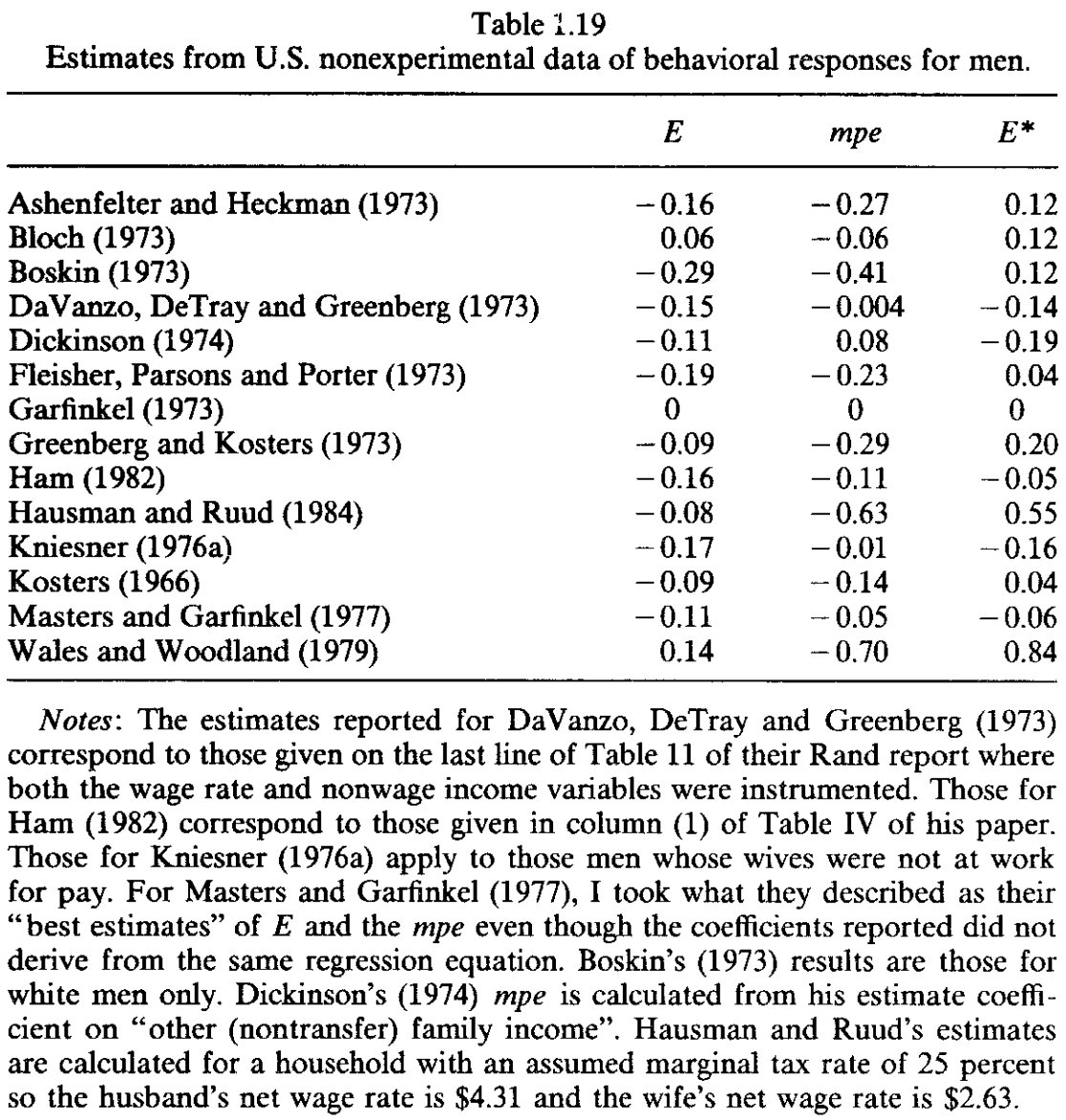
Source: Pencavel (1986)

Here, \(E\) refers to Marshallian elasticity \(\varepsilon_{hw}\), \(mpe\) - to income effect \(\frac{wh}{Y}\varepsilon_{hY}\) and \(E^\star\) - to Hicksian elasticity \(\eta_{hw}\).

• Large variation between different estimates

  • Marshallian elasticity between -0.29 and 0.14

  • Income effect from -0.70 to 0.08

  • Some even report negative Hicksian elasticity up to -0.19!

• These estimates are obtained from non-experimental survey datasets that are plagued by the issues mentioned above.

• To solve some of these issues, researchers turn to “experimental” data.

Estimates

Experimental data: drop in tax rates in the UK 1978-92

Source: Blundell, Duncan, and Meghir (1998)

It is very difficult to run a field experiment where researchers could vary wages completely exogenously and let workers decide on their labour supply.

Instead, many studies rely on quasi-experimental data. For example, Blundell, Duncan, and Meghir (1998) exploit change in tax rates in the UK. While the tax rate does not change gross wage, it does change net wage of workers. And it is unlikely that this policy change is correlated with individual characteristics of worker, i.e., it is exogenous. Therefore, by studying the behaviour of workers around the change allows us to draw inference about elasticity of their labour supply with respect to wages.

Notice that now Hicksian elasticities (in the second column) are all positive. These estimates are based on the behaviour of married women. It is also interesting that the labour supply elasticity rises considerably among mothers of young children. Can you think why? What can you say about data that is necessary for these estimations?

Are these values large? Some suggest participation is important, but overlooked in these studies!

Estimates

Intensive vs extensive margin

Source: Chetty et al. (2012)

Also some research on work effort for given hours of work (Dickinson 1999)

When wages change, workers may adjust both hours of work (intensive) and probability of working (extensive margin). Many studies have found extensive margin elasticities higher than intensive margin. There are two reasons for these findings

• Indivisible labour supply (Chetty et al. 2012)

  In the simple model, workers are allowed to choose any amount of hours worked between \(0\) and \(L_0\). In reality, we may not be able to adjust hours worked so freely. Often full-time employment contracts specify 8 hours of work, part-time contracts - may specify 4 hours of work a day. In this case, it makes sense that a small change in wages is unlikely to change hours worked in any meaningful way. What about quality of each hour worked? See Dickinson (1999). Instead, workers’ choices may be limited to participation and choice of contract (full-time/part-time). Thus, elasticity of participation is likely to be higher than that of hours worked, and we may need to observe generally larger changes in wages to detect adjustments along these margins.

• Optimization frictions (Chetty 2012)

  Alternatively, workers may be able to choose hours of work freely on the continuum \([0, L_0]\), but have to incur adjustment costs. That is, if they wish to change hours worked, they need to pay extra cost \(c\). Such adjustments costs can also create optimal behaviour where workers do not change hours of work in response to small wage variations, but are more likely to change probability of working.

Estimates

Measurement errors

Classical measurement error in \(w_{it}\) attenuates the estimate of \(\alpha_w\)

“Denominator bias” \(\downarrow \alpha_w\) if wages are computed as ratio of earning and hours with measurement errors. M. P. Keane (2011) computes average Hicksian elasticity

• among all papers: 0.31

• among papers with direct measure of \(w_{it}\): 0.43

Estimates

Measurement of consumption

PSID (US) dataset only includes food consumption data

Consumption measure	Marshall	Hicks	Income	Frisch
PSID unadjusted	-0.442	0.094	-0.536	0.148
Food + imputed (food prices, demographics)	-0.468	0.328	-0.796	0.535
Food + imputed (house value, rent)	-0.313	0.220	-0.533	0.246

Source: (M. P. Keane 2011, Table 5)

As mentioned above, many datasets do not have measures of total household expenditrures. For example, here is the survey of the results reported in papers that use PSID (Panel Study of Income Dynamics). The dataset only contains a variable that records food consumption data.

The first row shows the estimates of elasticities when only this variable is used for \(C_{it}\). In the second row, the \(C_{it}\) includes both actual food consumption and imputed consumption based on food prices and demographics. In the third row, the food consumption is complemented with imputed consumption based on house value and rent. The elasticities with adjusted \(C_{it}\) are considerably higher.

Estimates

Micro vs macro elasticities

Macro elasticities of labour supply typically higher than micro estimates

M. Keane and Rogerson (2012) highlight:

• extensive vs intensive margin
• model misspecification due to human capital accumulation
• aggregation is not straightforward

We have seen in the table reported by Chetty et al. (2012) also the difference between estimates of elasticities in the micro and macro data. Typically, the estimates from macro data deliver much higher elasticities.

There may be several possible explanations for the disparity.

• Again, the question of intensive and extensive margins. In macro data, aggregate hours worked depend on both, while in micro data hours worked can only be observed if a worker is employed.
• In the simple labour supply model we have not (yet) specified individual heterogeneity in human capital accumulation. These can also lead to different estimates as part of the changes in wages may be absorbed by human capital decisions.
• Finally, aggregating responses of workers in the economy may not be as straightforward as summing them up. The aggregate responses also depend on the responses of other sides of the market - firms and market structure.

Estimates

Discrete choice dynamic programming

Incorporate discrete choices into model of labour supply

• labour force participation (Eckstein and Wolpin 1989)
• marriage (Van Der Klaauw 1996)
• fertility (Francesconi 2002)

M. P. Keane and Wolpin (2010) combine all + school and welfare participation choices

Uncompensated dynamic elasticity

Eckstein and Wolpin (1989)	5.0
Van Der Klaauw (1996)	3.6
Francesconi (2002)	5.6
M. P. Keane and Wolpin (2010)	2.8

Source: M. P. Keane (2011)

We have seen earlier in the slides that

• inclusion of extensive and intensive margins of labour supply is important, and
• labour supply decisions may look different around the time of child birth, especially for women.

Therefore, one of the interesting extension of basic labour supply model incorporates marriage and fertility decisions. You can see that papers that include some or all of these features in their model, obtain estimates of labour supply elasticity much closer to the ones found in macro data.

Summary

• Standard models of labour supply
  • Static model
  • Household model
  • Intertemporal model
• Estimates of labour supply elasticities
  • Typical issues encountered in data
  • Variation in estimates and possible extensions
• Mostly covered seminal papers, but many ongoing works
  • Tax and benefit policies
  • Cross-wage elasticities

Next lecture: Labour Demand on 01 Sep

References

Blundell, Richard, Alan Duncan, and Costas Meghir. 1998. “Estimating Labor Supply Responses Using Tax Reforms.” Econometrica 66 (4): 827–61. https://doi.org/10.2307/2999575.

Blundell, Richard, and Thomas Macurdy. 1999. “Chapter 27 - Labor Supply: A Review of Alternative Approaches.” In Handbook of Labor Economics, edited by Orley C. Ashenfelter and David Card, 3:1559–1695. Elsevier. https://doi.org/10.1016/S1573-4463(99)03008-4.

Cahuc, Pierre. 2004. Labor Economics. Cambridge (Mass.): MIT Press.

Chetty, Raj. 2012. “Bounds on Elasticities with Optimization Frictions: A Synthesis of Micro and Macro Evidence on Labor Supply.” Econometrica 80 (3): 969–1018. https://www.jstor.org/stable/41493842.

Chetty, Raj, Adam Guren, Day Manoli, and Andrea Weber. 2012. “Does Indivisible Labor Explain the Difference Between Micro and Macro Elasticities? A Meta-Analysis of Extensive Margin Elasticities.” NBER Macroeconomics Annual 27: 1–56. https://doi.org/10.1086/669170.

Chiappori, Pierre-André. 1992. “Collective Labor Supply and Welfare.” Journal of Political Economy 100 (3): 437–67. https://www.jstor.org/stable/2138727.

Dickinson, David L. 1999. “An Experimental Examination of Labor Supply and Work Intensities.” Journal of Labor Economics 17 (4): 638–70. https://doi.org/10.1086/209934.

Eckstein, Zvi, and Kenneth I. Wolpin. 1989. “Dynamic Labour Force Participation of Married Women and Endogenous Work Experience.” The Review of Economic Studies 56 (3): 375–90. https://doi.org/10.2307/2297553.

Francesconi, Marco. 2002. “A Joint Dynamic Model of Fertility and Work of Married Women.” Journal of Labor Economics 20 (2): 336–80. https://doi.org/10.1086/338220.

Keane, Michael P. 2011. “Labor Supply and Taxes: A Survey.” Journal of Economic Literature 49 (4): 961–1075. https://doi.org/10.1257/jel.49.4.961.

Keane, Michael P., and Kenneth I. Wolpin. 2010. “The Role of Labor and Marriage Markets, Preference Heterogeneity, and the Welfare System in the Life Cycle Decisions of Black, Hispanic, and White Women.” International Economic Review 51 (3): 851–92. https://www.jstor.org/stable/40784808.

Keane, Michael, and Richard Rogerson. 2012. “Micro and Macro Labor Supply Elasticities: A Reassessment of Conventional Wisdom.” Journal of Economic Literature 50 (2): 464–76. https://doi.org/10.1257/jel.50.2.464.

Lundberg, Shelly J., Robert A. Pollak, and Terence J. Wales. 1997. “Do Husbands and Wives Pool Their Resources? Evidence from the United Kingdom Child Benefit.” The Journal of Human Resources 32 (3): 463–80. https://doi.org/10.2307/146179.

Pencavel, John. 1986. “Chapter 1 Labor Supply of Men: A Survey.” In Handbook of Labor Economics, 1:3–102. Elsevier. https://doi.org/10.1016/S1573-4463(86)01004-0.

Ramey, Valerie A., and Neville Francis. 2009. “A Century of Work and Leisure.” American Economic Journal: Macroeconomics 1 (2): 189–224. https://doi.org/10.1257/mac.1.2.189.

Van Der Klaauw, Wilbert. 1996. “Female Labour Supply and Marital Status Decisions: A Life-Cycle Model.” The Review of Economic Studies 63 (2): 199–235. https://doi.org/10.2307/2297850.